Chapter 7 Expected value

This chapter deals with expected values of random variables.

The students are expected to acquire the following knowledge:

Theoretical

Calculation of the expected value.
Calculation of variance and covariance.
Cauchy distribution.

Estimation of expected value.
Estimation of variance and covariance.

7.1 Discrete random variables

Exercise 7.1 (Bernoulli) Let $X \sim \text{Bernoulli}(p)$.

Find $E[X]$.
Find $Var[X]$.
R: Let $p = 0.4$. Check your answers to a) and b) with a simulation.

Solution.

\[\begin{align*} E[X] = \sum_{k=0}^1 p^k (1-p)^{1-k} k = p. \end{align*}\]
\[\begin{align*} Var[X] = E[X^2] - E[X]^2 = \sum_{k=0}^1 (p^k (1-p)^{1-k} k^2) - p^2 = p(1-p). \end{align*}\]

set.seed(1)
nsamps <- 1000
x      <- rbinom(nsamps, 1, 0.4)
mean(x)

## [1] 0.394

var(x)

## [1] 0.239003

0.4 * (1 - 0.4)

## [1] 0.24

Exercise 7.2 (Binomial) Let $X \sim \text{Binomial}(n,p)$.

Find $E[X]$.
Find $Var[X]$.

Solution.

Let $X = \sum_{i=0}^n X_i$, where $X_i \sim \text{Bernoulli}(p)$. Then, due to linearity of expectation \[\begin{align*} E[X] = E[\sum_{i=0}^n X_i] = \sum_{i=0}^n E[X_i] = np. \end{align*}\]
Again let $X = \sum_{i=0}^n X_i$, where $X_i \sim \text{Bernoulli}(p)$. Since the Bernoulli variables $X_i$ are independent we have \[\begin{align*} Var[X] = Var[\sum_{i=0}^n X_i] = \sum_{i=0}^n Var[X_i] = np(1-p). \end{align*}\]

Exercise 7.3 (Poisson) Let $X \sim \text{Poisson}(\lambda)$.

Find $E[X]$.
Find $Var[X]$.

Solution.

\[\begin{align*} E[X] &= \sum_{k=0}^\infty \frac{\lambda^k e^{-\lambda}}{k!} k & \\ &= \sum_{k=1}^\infty \frac{\lambda^k e^{-\lambda}}{k!} k & \text{term at $k=0$ is 0} \\ &= e^{-\lambda} \lambda \sum_{k=1}^\infty \frac{\lambda^{k-1}}{(k - 1)!} & \\ &= e^{-\lambda} \lambda \sum_{k=0}^\infty \frac{\lambda^{k}}{k!} & \\ &= e^{-\lambda} \lambda e^\lambda & \\ &= \lambda. \end{align*}\]
\[\begin{align*} Var[X] &= E[X^2] - E[X]^2 & \\ &= e^{-\lambda} \lambda \sum_{k=1}^\infty k \frac{\lambda^{k-1}}{(k - 1)!} - \lambda^2 & \\ &= e^{-\lambda} \lambda \sum_{k=1}^\infty (k - 1) + 1) \frac{\lambda^{k-1}}{(k - 1)!} - \lambda^2 & \\ &= e^{-\lambda} \lambda \big(\sum_{k=1}^\infty (k - 1) \frac{\lambda^{k-1}}{(k - 1)!} + \sum_{k=1}^\infty \frac{\lambda^{k-1}}{(k - 1)!}\Big) - \lambda^2 & \\ &= e^{-\lambda} \lambda \big(\lambda\sum_{k=2}^\infty \frac{\lambda^{k-2}}{(k - 2)!} + e^\lambda\Big) - \lambda^2 & \\ &= e^{-\lambda} \lambda \big(\lambda e^\lambda + e^\lambda\Big) - \lambda^2 & \\ &= \lambda^2 + \lambda - \lambda^2 & \\ &= \lambda. \end{align*}\]

Exercise 7.4 (Geometric) Let $X \sim \text{Geometric}(p)$.

Find $E[X]$. Hint: $\frac{d}{dx} x^k = k x^{(k - 1)}$.

Solution.

\[\begin{align*} E[X] &= \sum_{k=0}^\infty (1 - p)^k p k & \\ &= p (1 - p) \sum_{k=0}^\infty (1 - p)^{k-1} k & \\ &= p (1 - p) \sum_{k=0}^\infty -\frac{d}{dp}(1 - p)^k & \\ &= p (1 - p) \Big(-\frac{d}{dp}\Big) \sum_{k=0}^\infty (1 - p)^k & \\ &= p (1 - p) \Big(-\frac{d}{dp}\Big) \frac{1}{1 - (1 - p)} & \text{geometric series} \\ &= \frac{1 - p}{p} \end{align*}\]

7.2 Continuous random variables

Exercise 7.5 (Gamma) Let $X \sim \text{Gamma}(\alpha, \beta)$. Hint: $\Gamma(z) = \int_0^\infty t^{z-1}e^{-t} dt$ and $\Gamma(z + 1) = z \Gamma(z)$.

Find $E[X]$.
Find $Var[X]$.
R: Let $\alpha = 10$ and $\beta = 2$. Plot the density of $X$. Add a horizontal line at the expected value that touches the density curve (geom_segment). Shade the area within a standard deviation of the expected value.

Solution.

\[\begin{align*} E[X] &= \int_0^\infty \frac{\beta^\alpha}{\Gamma(\alpha)}x^\alpha e^{-\beta x} dx & \\ &= \frac{\beta^\alpha}{\Gamma(\alpha)} \int_0^\infty x^\alpha e^{-\beta x} dx & \text{ (let $t = \beta x$)} \\ &= \frac{\beta^\alpha}{\Gamma(\alpha) }\int_0^\infty \frac{t^\alpha}{\beta^\alpha} e^{-t} \frac{dt}{\beta} & \\ &= \frac{1}{\beta \Gamma(\alpha) }\int_0^\infty t^\alpha e^{-t} dt & \\ &= \frac{\Gamma(\alpha + 1)}{\beta \Gamma(\alpha)} & \\ &= \frac{\alpha \Gamma(\alpha)}{\beta \Gamma(\alpha)} & \\ &= \frac{\alpha}{\beta}. & \end{align*}\]
\[\begin{align*} Var[X] &= E[X^2] - E[X]^2 \\ &= \int_0^\infty \frac{\beta^\alpha}{\Gamma(\alpha)}x^{\alpha+1} e^{-\beta x} dx - \frac{\alpha^2}{\beta^2} \\ &= \frac{\Gamma(\alpha + 2)}{\beta^2 \Gamma(\alpha)} - \frac{\alpha^2}{\beta^2} \\ &= \frac{(\alpha + 1)\alpha\Gamma(\alpha)}{\beta^2 \Gamma(\alpha)} - \frac{\alpha^2}{\beta^2} \\ &= \frac{\alpha^2 + \alpha}{\beta^2} - \frac{\alpha^2}{\beta^2} \\ &= \frac{\alpha}{\beta^2}. \end{align*}\]

set.seed(1)
x  <- seq(0, 25, by = 0.01)
y  <- dgamma(x, shape = 10, rate = 2)
df <- data.frame(x = x, y = y)
ggplot(df, aes(x = x, y = y)) +
  geom_line() +
  geom_segment(aes(x = 5, y = 0, xend = 5,
                   yend = dgamma(5, shape = 10, rate = 2)),
               color = "red") +
  stat_function(fun = dgamma, args = list(shape = 10, rate = 2), 
                xlim = c(5 - sqrt(10/4), 5 + sqrt(10/4)), geom = "area", fill = "gray", alpha = 0.4)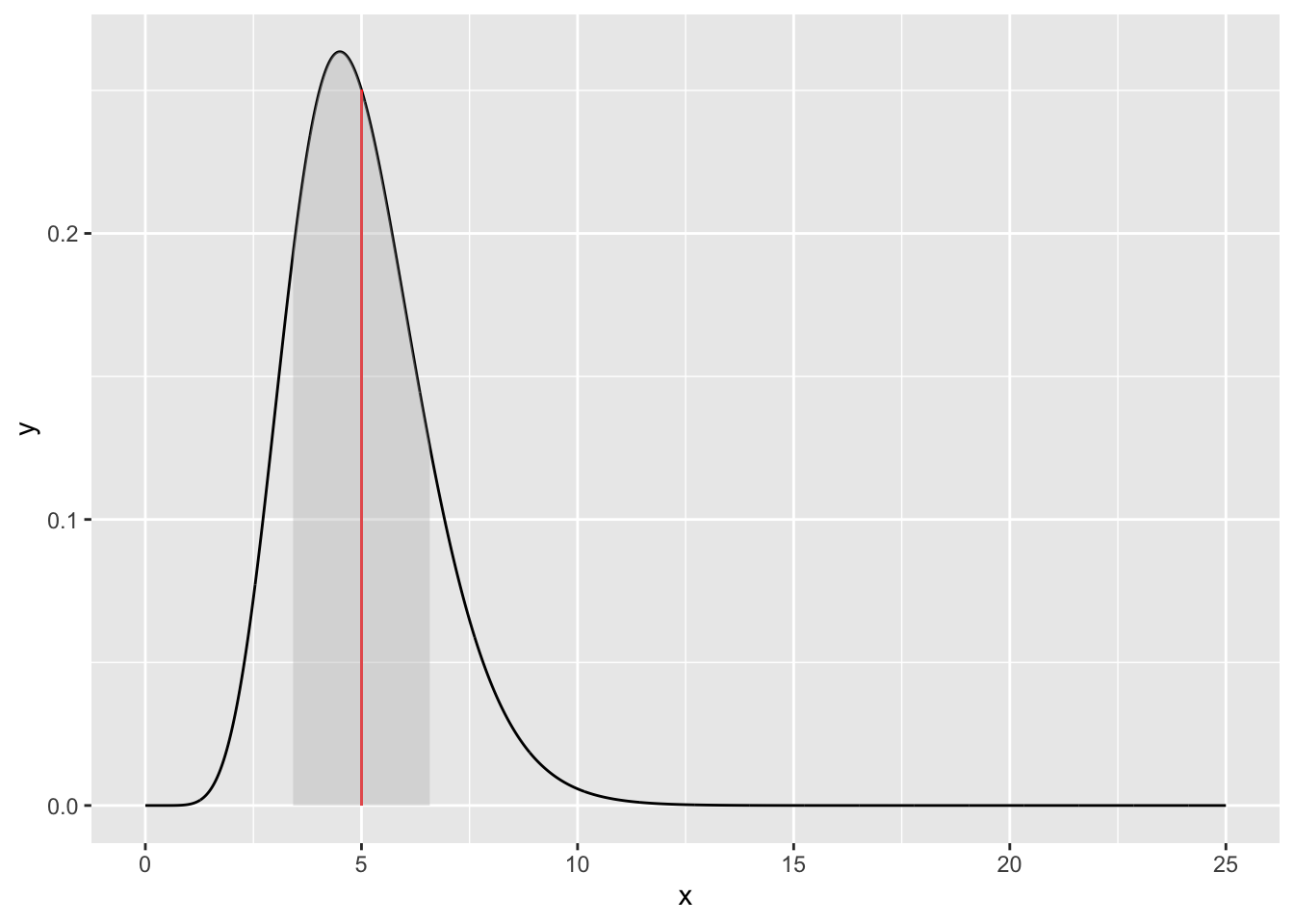

Exercise 7.6 (Beta) Let $X \sim \text{Beta}(\alpha, \beta)$.

Find $E[X]$. Hint 1: $\text{B}(x,y) = \int_0^1 t^{x-1} (1 - t)^{y-1} dt$. Hint 2: $\text{B}(x + 1, y) = \text{B}(x,y)\frac{x}{x + y}$.
Find $Var[X]$.

Solution.

\[\begin{align*} E[X] &= \int_0^1 \frac{x^{\alpha - 1} (1 - x)^{\beta - 1}}{\text{B}(\alpha, \beta)} x dx \\ &= \frac{1}{\text{B}(\alpha, \beta)}\int_0^1 x^{\alpha} (1 - x)^{\beta - 1} dx \\ &= \frac{1}{\text{B}(\alpha, \beta)} \text{B}(\alpha + 1, \beta) \\ &= \frac{1}{\text{B}(\alpha, \beta)} \text{B}(\alpha, \beta) \frac{\alpha}{\alpha + \beta} \\ &= \frac{\alpha}{\alpha + \beta}. \\ \end{align*}\]
\[\begin{align*} Var[X] &= E[X^2] - E[X]^2 \\ &= \int_0^1 \frac{x^{\alpha - 1} (1 - x)^{\beta - 1}}{\text{B}(\alpha, \beta)} x^2 dx - \frac{\alpha^2}{(\alpha + \beta)^2} \\ &= \frac{1}{\text{B}(\alpha, \beta)}\int_0^1 x^{\alpha + 1} (1 - x)^{\beta - 1} dx - \frac{\alpha^2}{(\alpha + \beta)^2} \\ &= \frac{1}{\text{B}(\alpha, \beta)} \text{B}(\alpha + 2, \beta) - \frac{\alpha^2}{(\alpha + \beta)^2} \\ &= \frac{1}{\text{B}(\alpha, \beta)} \text{B}(\alpha + 1, \beta) \frac{\alpha + 1}{\alpha + \beta + 1} - \frac{\alpha^2}{(\alpha + \beta)^2} \\ &= \frac{\alpha + 1}{\alpha + \beta + 1} \frac{\alpha}{\alpha + \beta} - \frac{\alpha^2}{(\alpha + \beta)^2}\\ &= \frac{\alpha \beta}{(\alpha + \beta)^2(\alpha + \beta + 1)}. \end{align*}\]

Exercise 7.7 (Exponential) Let $X \sim \text{Exp}(\lambda)$.

Find $E[X]$. Hint: $\Gamma(z + 1) = z\Gamma(z)$ and $\Gamma(1) = 1$.
Find $Var[X]$.

Solution.

\[\begin{align*} E[X] &= \int_0^\infty \lambda e^{-\lambda x} x dx & \\ &= \lambda \int_0^\infty x e^{-\lambda x} dx & \\ &= \lambda \int_0^\infty \frac{t}{\lambda} e^{-t} \frac{dt}{\lambda} & \text{$t = \lambda x$}\\ &= \lambda \lambda^{-2} \Gamma(2) & \text{definition of gamma function} \\ &= \lambda^{-1}. \end{align*}\]
\[\begin{align*} Var[X] &= E[X^2] - E[X]^2 & \\ &= \int_0^\infty \lambda e^{-\lambda x} x^2 dx - \lambda^{-2} & \\ &= \lambda \int_0^\infty \frac{t^2}{\lambda^2} e^{-t} \frac{dt}{\lambda} - \lambda^{-2} & \text{$t = \lambda x$} \\ &= \lambda \lambda^{-3} \Gamma(3) - \lambda^{-2} & \text{definition of gamma function} & \\ &= \lambda^{-2} 2 \Gamma(2) - \lambda^{-2} & \\ &= 2 \lambda^{-2} - \lambda^{-2} & \\ &= \lambda^{-2}. & \\ \end{align*}\]

Exercise 7.8 (Normal) Let $X \sim \text{N}(\mu, \sigma)$.

Show that $E[X] = \mu$. Hint: Use the error function $\text{erf}(x) = \frac{1}{\sqrt(\pi)} \int_{-x}^x e^{-t^2} dt$. The statistical interpretation of this function is that if $Y \sim \text{N}(0, 0.5)$, then the error function describes the probability of $Y$ falling between $-x$ and $x$. Also, $\text{erf}(\infty) = 1$.
Show that $Var[X] = \sigma^2$. Hint: Start with the definition of variance.

Solution.

\[\begin{align*} E[X] &= \int_{-\infty}^\infty \frac{1}{\sqrt{2\pi \sigma^2}} e^{-\frac{(x - \mu)^2}{2\sigma^2}} x dx & \\ &= \frac{1}{\sqrt{2\pi \sigma^2}} \int_{-\infty}^\infty x e^{-\frac{(x - \mu)^2}{2\sigma^2}} dx & \\ &= \frac{1}{\sqrt{2\pi \sigma^2}} \int_{-\infty}^\infty \Big(t \sqrt{2\sigma^2} + \mu\Big)e^{-t^2} \sqrt{2 \sigma^2} dt & t = \frac{x - \mu}{\sqrt{2}\sigma} \\ &= \frac{\sqrt{2\sigma^2}}{\sqrt{\pi}} \int_{-\infty}^\infty t e^{-t^2} dt + \frac{1}{\sqrt{\pi}} \int_{-\infty}^\infty \mu e^{-t^2} dt & \\ \end{align*}\]

Let us calculate these integrals separately. \[\begin{align*} \int t e^{-t^2} dt &= -\frac{1}{2}\int e^{s} ds & s = -t^2 \\ &= -\frac{e^s}{2} + C \\ &= -\frac{e^{-t^2}}{2} + C & \text{undoing substitution}. \end{align*}\] Inserting the integration limits we get \[\begin{align*} \int_{-\infty}^\infty t e^{-t^2} dt &= 0, \end{align*}\] due to the integrated function being symmetric.

Reordering the second integral we get \[\begin{align*} \mu \frac{1}{\sqrt{\pi}} \int_{-\infty}^\infty e^{-t^2} dt &= \mu \text{erf}(\infty) & \text{definition of error function} \\ &= \mu & \text{probability of $Y$ falling between $-\infty$ and $\infty$}. \end{align*}\] Combining all of the above we get \[\begin{align*} E[X] &= \frac{\sqrt{2\sigma^2}}{\sqrt{\pi}} \times 0 + \mu &= \mu.\\ \end{align*}\]

\[\begin{align*} Var[X] &= E[(X - E[X])^2] \\ &= E[(X - \mu)^2] \\ &= \frac{1}{\sqrt{2\pi \sigma^2}} \int_{-\infty}^\infty (x - \mu)^2 e^{-\frac{(x - \mu)^2}{2\sigma^2}} dx \\ &= \frac{\sigma^2}{\sqrt{2\pi}} \int_{-\infty}^\infty t^2 e^{-\frac{t^2}{2}} dt \\ &= \frac{\sigma^2}{\sqrt{2\pi}} \bigg(\Big(- t e^{-\frac{t^2}{2}} |_{-\infty}^\infty \Big) + \int_{-\infty}^\infty e^{-\frac{t^2}{2}} \bigg) dt & \text{integration by parts} \\ &= \frac{\sigma^2}{\sqrt{2\pi}} \sqrt{2 \pi} \int_{-\infty}^\infty \frac{1}{\sqrt(\pi)}e^{-s^2} \bigg) & s = \frac{t}{\sqrt{2}} \text{ and evaluating the left expression at the bounds} \\ &= \frac{\sigma^2}{\sqrt{2\pi}} \sqrt{2 \pi} \Big(\text{erf}(\infty) & \text{definition of error function} \\ &= \sigma^2. \end{align*}\]

7.3 Sums, functions, conditional expectations

Exercise 7.9 (Expectation of transformations) Let $X$ follow a normal distribution with mean $\mu$ and variance $\sigma^2$.

Find $E[2X + 4]$.
Find $E[X^2]$.
Find $E[\exp(X)]$. Hint: Use the error function $\text{erf}(x) = \frac{1}{\sqrt(\pi)} \int_{-x}^x e^{-t^2} dt$. Also, $\text{erf}(\infty) = 1$.
R: Check your results numerically for $\mu = 0.4$ and $\sigma^2 = 0.25$ and plot the densities of all four distributions.

Solution.

\[\begin{align} E[2X + 4] &= 2E[X] + 4 & \text{linearity of expectation} \\ &= 2\mu + 4. \\ \end{align}\]
\[\begin{align} E[X^2] &= E[X]^2 + Var[X] & \text{definition of variance} \\ &= \mu^2 + \sigma^2. \end{align}\]
\[\begin{align} E[\exp(X)] &= \int_{-\infty}^\infty \frac{1}{\sqrt{2\pi \sigma^2}} e^{-\frac{(x - \mu)^2}{2\sigma^2}} e^x dx & \\ &= \frac{1}{\sqrt{2\pi \sigma^2}} \int_{-\infty}^\infty e^{\frac{2 \sigma^2 x}{2\sigma^2} -\frac{(x - \mu)^2}{2\sigma^2}} dx & \\ &= \frac{1}{\sqrt{2\pi \sigma^2}} \int_{-\infty}^\infty e^{-\frac{x^2 - 2x(\mu + \sigma^2) + \mu^2}{2\sigma^2}} dx & \\ &= \frac{1}{\sqrt{2\pi \sigma^2}} \int_{-\infty}^\infty e^{-\frac{(x - (\mu + \sigma^2))^2 + \mu^2 - (\mu + \sigma^2)^2}{2\sigma^2}} dx & \text{complete the square} \\ &= \frac{1}{\sqrt{2\pi \sigma^2}} e^{\frac{- \mu^2 + (\mu + \sigma^2)^2}{2\sigma^2}} \int_{-\infty}^\infty e^{-\frac{(x - (\mu + \sigma^2))^2}{2\sigma^2}} dx & \\ &= \frac{1}{\sqrt{2\pi \sigma^2}} e^{\frac{- \mu^2 + (\mu + \sigma^2)^2}{2\sigma^2}} \sigma \sqrt{2 \pi} \text{erf}(\infty) & \\ &= e^{\frac{2\mu + \sigma^2}{2}}. \end{align}\]

set.seed(1)
mu    <- 0.4
sigma <- 0.5
x     <- rnorm(100000, mean = mu, sd = sigma)

mean(2*x + 4)

## [1] 4.797756

2 * mu + 4

## [1] 4.8

mean(x^2)

## [1] 0.4108658

mu^2 + sigma^2

## [1] 0.41

mean(exp(x))

## [1] 1.689794

exp((2 * mu + sigma^2) / 2)

## [1] 1.690459

Exercise 7.10 (Sum of independent random variables) Borrowed from Wasserman. Let $X_1, X_2,...,X_n$ be IID random variables with expected value $E[X_i] = \mu$ and variance $Var[X_i] = \sigma^2$. Find the expected value and variance of $\bar{X} = \frac{1}{n} \sum_{i=1}^n X_i$. $\bar{X}$ is called a statistic (a function of the values in a sample). It is itself a random variable and its distribution is called a sampling distribution. R: Take $n = 5, 10, 100, 1000$ samples from the N($2$, $6$) distribution 10000 times. Plot the theoretical density and the densities of $\bar{X}$ statistic for each $n$. Intuitively, are the results in correspondence with your calculations? Check them numerically.

Solution. Let us start with the expectation of $\bar{X}$.

\[\begin{align} E[\bar{X}] &= E[\frac{1}{n} \sum_{i=1}^n X_i] & \\ &= \frac{1}{n} E[\sum_{i=1}^n X_i] & \text{ (multiplication with a scalar)} \\ &= \frac{1}{n} \sum_{i=1}^n E[X_i] & \text{ (linearity)} \\ &= \frac{1}{n} n \mu & \\ &= \mu. \end{align}\]

Now the variance \[\begin{align} Var[\bar{X}] &= Var[\frac{1}{n} \sum_{i=1}^n X_i] & \\ &= \frac{1}{n^2} Var[\sum_{i=1}^n X_i] & \text{ (multiplication with a scalar)} \\ &= \frac{1}{n^2} \sum_{i=1}^n Var[X_i] & \text{ (independence of samples)} \\ &= \frac{1}{n^2} n \sigma^2 & \\ &= \frac{1}{n} \sigma^2. \end{align}\]

set.seed(1)
nsamps <- 10000
mu     <- 2
sigma  <- sqrt(6)
N      <- c(5, 10, 100, 500)
X      <- matrix(data = NA, nrow = nsamps, ncol = length(N))
ind    <- 1
for (n in N) {
  for (i in 1:nsamps) {
    X[i,ind] <- mean(rnorm(n, mu, sigma))
  }
  ind <- ind + 1
}
colnames(X) <- N
X           <- melt(as.data.frame(X))

ggplot(data = X, aes(x = value, colour = variable)) +
  geom_density() +
  stat_function(data  = data.frame(x = seq(-2, 6, by = 0.01)), aes(x = x), 
                fun   = dnorm, 
                args  = list(mean = mu, sd = sigma), 
                color = "black")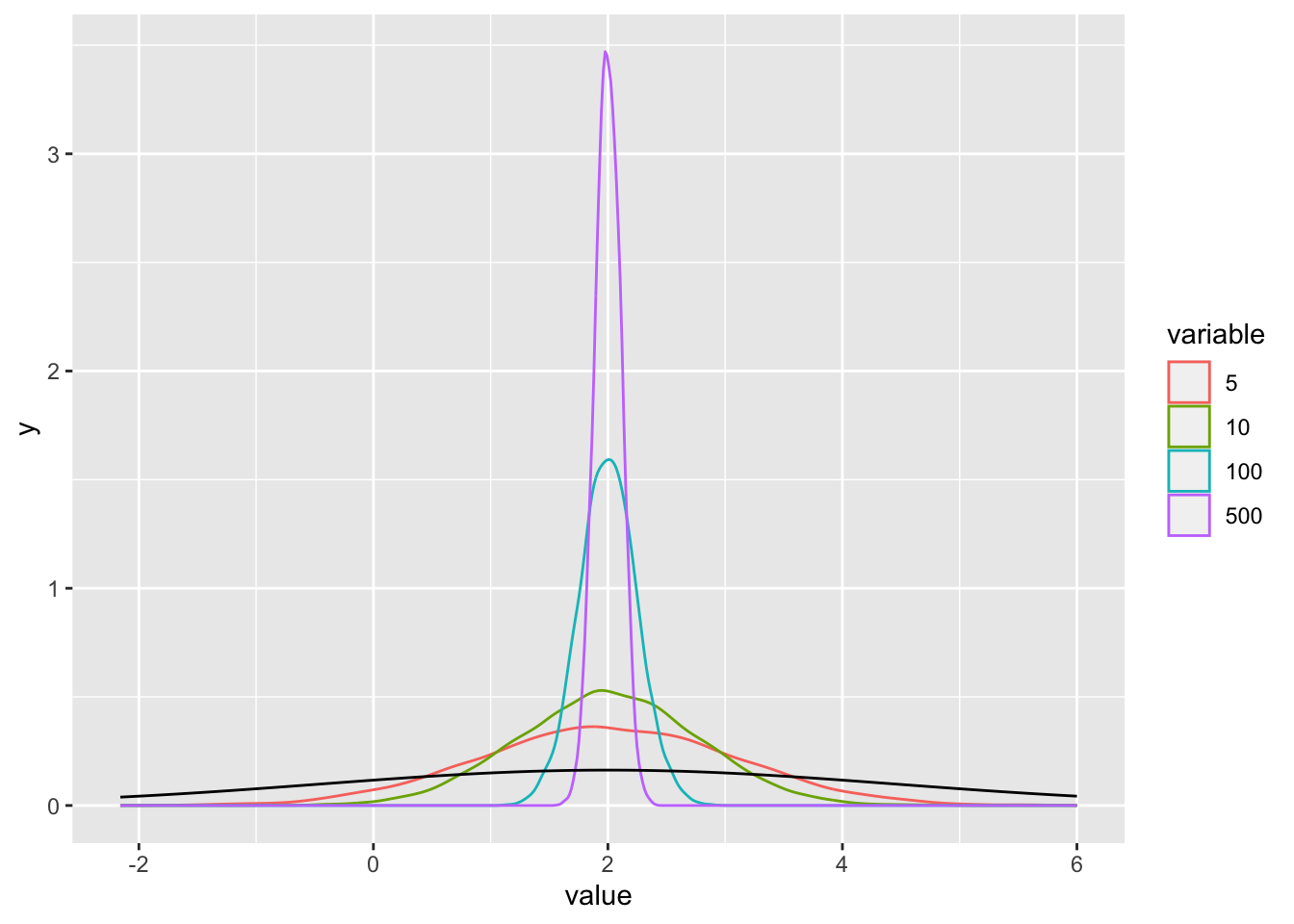

Exercise 7.11 (Conditional expectation) Let $X \in \mathbb{R}_0^+$ and $Y \in \mathbb{N}_0$ be random variables with joint distribution $p_{XY}(X,Y) = \frac{1}{y + 1} e^{-\frac{x}{y + 1}} 0.5^{y + 1}$.

Find $E[X | Y = y]$ by first finding $p_Y$ and then $p_{X|Y}$.
Find $E[X]$.
R: check your answers to a) and b) by drawing 10000 samples from $p_Y$ and $p_{X|Y}$.

Solution.

\[\begin{align} p(y) &= \int_0^\infty \frac{1}{y + 1} e^{-\frac{x}{y + 1}} 0.5^{y + 1} dx \\ &= \frac{0.5^{y + 1}}{y + 1} \int_0^\infty e^{-\frac{x}{y + 1}} dx \\ &= \frac{0.5^{y + 1}}{y + 1} (y + 1) \\ &= 0.5^{y + 1} \\ &= 0.5(1 - 0.5)^y. \end{align}\] We recognize this as the geometric distribution. \[\begin{align} p(x|y) &= \frac{p(x,y)}{p(y)} \\ &= \frac{1}{y + 1} e^{-\frac{x}{y + 1}}. \end{align}\] We recognize this as the exponential distribution. \[\begin{align} E[X | Y = y] &= \int_0^\infty x \frac{1}{y + 1} e^{-\frac{x}{y + 1}} dx \\ &= y + 1 & \text{expected value of the exponential distribution} \end{align}\]
Use the law of iterated expectation. \[\begin{align} E[X] &= E[E[X | Y]] \\ &= E[Y + 1] \\ &= E[Y] + 1 \\ &= \frac{1 - 0.5}{0.5} + 1 \\ &= 2. \end{align}\]

set.seed(1)
y  <- rgeom(100000, 0.5)
x  <- rexp(100000, rate = 1 / (y + 1))
x2 <- x[y == 3]

mean(x2)

## [1] 4.048501

3 + 1

## [1] 4

mean(x)

## [1] 2.007639

(1 - 0.5) / 0.5 + 1

## [1] 2

Exercise 7.12 (Cauchy distribution) Let $p(x | x_0, \gamma) = \frac{1}{\pi \gamma \Big(1 + \big(\frac{x - x_0}{\gamma}\big)^2\Big)}$. A random variable with this PDF follows a Cauchy distribution. This distribution is symmetric and has wider tails than the normal distribution.

R: Draw $n = 1,...,1000$ samples from a standard normal and $\text{Cauchy}(0, 1)$. For each $n$ plot the mean and the median of the sample using facets. Interpret the results.
To get a mathematical explanation of the results in a), evaluate the integral $\int_0^\infty \frac{x}{1 + x^2} dx$ and consider that $E[X] = \int_{-\infty}^\infty \frac{x}{1 + x^2}dx$.

set.seed(1)
n         <- 1000
means_n   <- vector(mode = "numeric", length = n)
means_c   <- vector(mode = "numeric", length = n)
medians_n <- vector(mode = "numeric", length = n)
medians_c <- vector(mode = "numeric", length = n)
for (i in 1:n) {
  tmp_n        <- rnorm(i)
  tmp_c        <- rcauchy(i)
  means_n[i]   <- mean(tmp_n)
  means_c[i]   <- mean(tmp_c)
  medians_n[i] <- median(tmp_n)
  medians_c[i] <- median(tmp_c)
}
df <- data.frame("distribution" = c(rep("normal", 2 * n),
                                    rep("Cauchy", 2 * n)),
                 "type"         = c(rep("mean", n),
                                    rep("median", n),
                                    rep("mean", n),
                                    rep("median", n)),
                 "value"        = c(means_n, medians_n, means_c, medians_c),
                 "n"            = rep(1:n, times = 4))
ggplot(df, aes(x = n, y = value)) +
  geom_line(alpha = 0.5) +
  facet_wrap(~ type + distribution , scales = "free")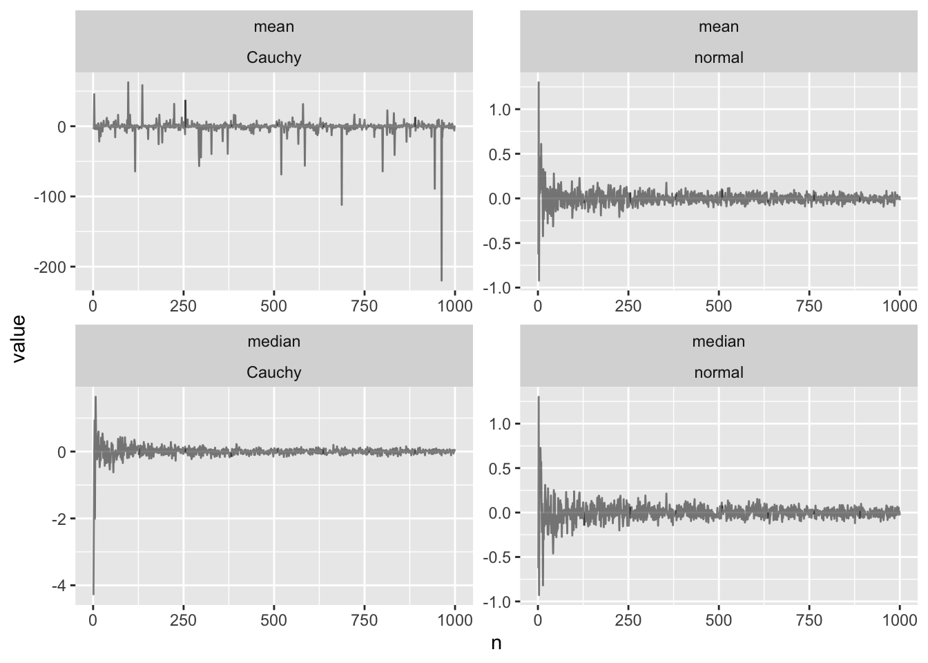

Solution.

\[\begin{align} \int_0^\infty \frac{x}{1 + x^2} dx &= \frac{1}{2} \int_1^\infty \frac{1}{u} du & u = 1 + x^2 \\ &= \frac{1}{2} \ln(x) |_0^\infty. \end{align}\]

This integral is not finite. The same holds for the negative part. Therefore, the expectation is undefined, as $E[|X|] = \infty$.

Why can we not just claim that $f(x) = x / (1 + x^2)$ is odd and $\int_{-\infty}^\infty f(x) = 0$? By definition of the Lebesgue integral $\int_{-\infty}^{\infty} f= \int_{-\infty}^{\infty} f_+-\int_{-\infty}^{\infty} f_-$. At least one of the two integrals needs to be finite for $\int_{-\infty}^{\infty} f$ to be well-defined. However $\int_{-\infty}^{\infty} f_+=\int_0^{\infty} x/(1+x^2)$ and $\int_{-\infty}^{\infty} f_-=\int_{-\infty}^{0} |x|/(1+x^2)$. We have just shown that both of these integrals are infinite, which implies that their sum is also infinite.

7.4 Covariance

Exercise 7.13 Below is a table of values for random variables $X$ and $Y$.

X	Y
2.1	8
-0.5	11
1	10
-2	12
4	9

Find sample covariance of $X$ and $Y$.
Find sample variances of $X$ and $Y$.
Find sample correlation of $X$ and $Y$.
Find sample variance of $Z = 2X - 3Y$.

Solution.

$\bar{X} = 0.92$ and $\bar{Y} = 10$. \[\begin{align} s(X, Y) &= \frac{1}{n - 1} \sum_{i=1}^5 (X_i - 0.92) (Y_i - 10) \\ &= -3.175. \end{align}\]
\[\begin{align} s(X) &= \frac{\sum_{i=1}^5(X_i - 0.92)^2}{5 - 1} \\ &= 5.357. \end{align}\] \[\begin{align} s(Y) &= \frac{\sum_{i=1}^5(Y_i - 10)^2}{5 - 1} \\ &= 2.5. \end{align}\]
\[\begin{align} r(X,Y) &= \frac{Cov(X,Y)}{\sqrt{Var[X]Var[Y]}} \\ &= \frac{-3.175}{\sqrt{5.357 \times 2.5}} \\ &= -8.68. \end{align}\]
\[\begin{align} s(Z) &= 2^2 s(X) + 3^2 s(Y) + 2 \times 2 \times 3 s(X, Y) \\ &= 4 \times 5.357 + 9 \times 2.5 + 12 \times 3.175 \\ &= 82.028. \end{align}\]

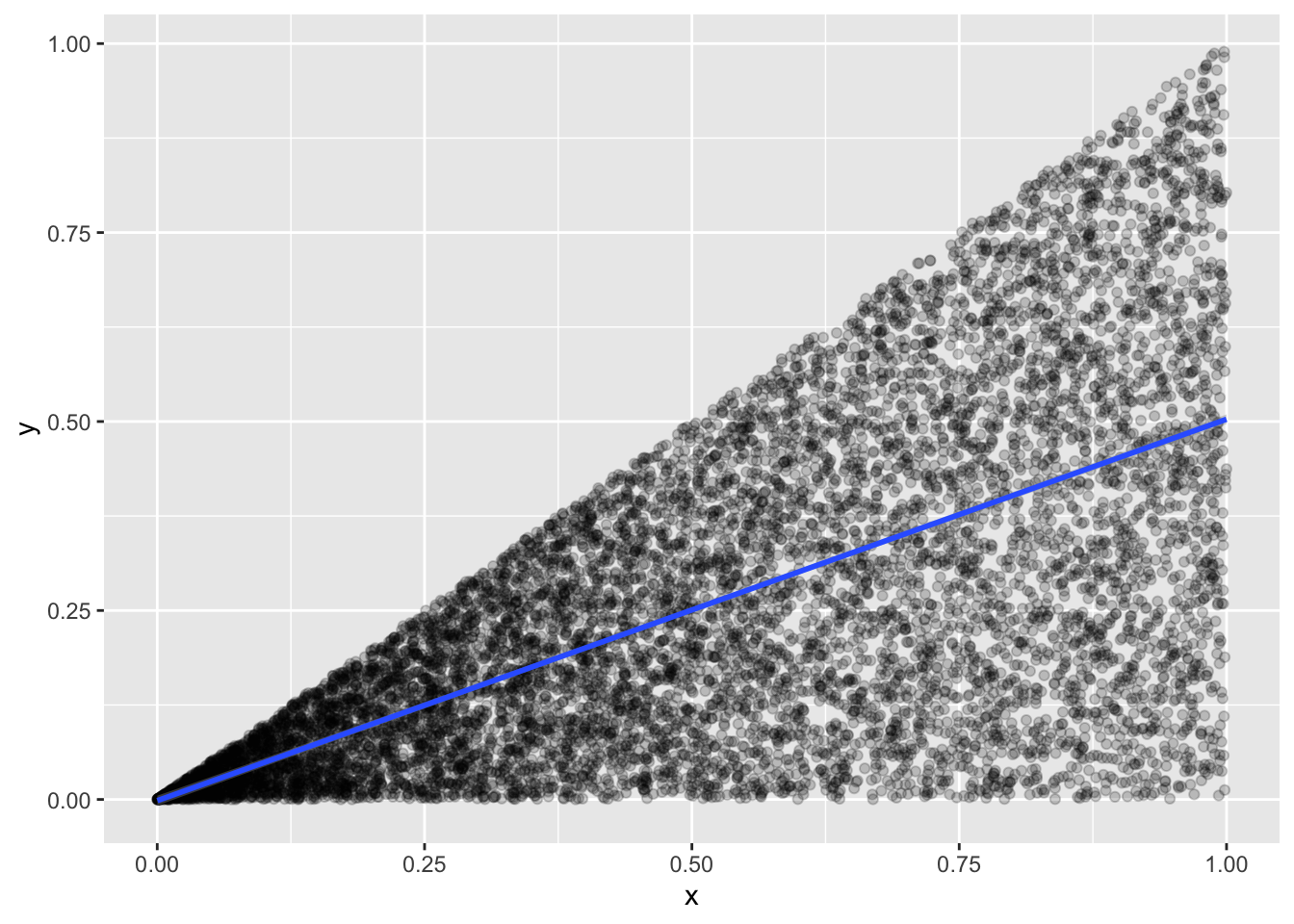
Exercise 7.14 Let $X \sim \text{Uniform}(0,1)$ and $Y | X = x \sim \text{Uniform(0,x)}$.

Find the covariance of $X$ and $Y$.
Find the correlation of $X$ and $Y$.
R: check your answers to a) and b) with simulation. Plot $X$ against $Y$ on a scatterplot.

Solution.

The joint PDF is $p(x,y) = p(x)p(y|x) = \frac{1}{x}$. \[\begin{align} Cov(X,Y) &= E[XY] - E[X]E[Y] \\ \end{align}\] Let us first evaluate the first term: \[\begin{align} E[XY] &= \int_0^1 \int_0^x x y \frac{1}{x} dy dx \\ &= \int_0^1 \int_0^x y dy dx \\ &= \int_0^1 \frac{x^2}{2} dx \\ &= \frac{1}{6}. \end{align}\] Now let us find $E[Y]$, $E[X]$ is trivial. \[\begin{align} E[Y] = E[E[Y | X]] = E[\frac{X}{2}] = \frac{1}{2} \int_0^1 x dx = \frac{1}{4}. \end{align}\] Combining all: \[\begin{align} Cov(X,Y) &= \frac{1}{6} - \frac{1}{2} \frac{1}{4} = \frac{1}{24}. \end{align}\]
\[\begin{align} \rho(X,Y) &= \frac{Cov(X,Y)}{\sqrt{Var[X]Var[Y]}} \\ \end{align}\] Let us calculate $Var[X]$. \[\begin{align} Var[X] &= E[X^2] - \frac{1}{4} \\ &= \int_0^1 x^2 - \frac{1}{4} \\ &= \frac{1}{3} - \frac{1}{4} \\ &= \frac{1}{12}. \end{align}\] Let us calculate $E[E[Y^2|X]]$. \[\begin{align} E[E[Y^2|X]] &= E[\frac{x^2}{3}] \\ &= \frac{1}{9}. \end{align}\] Then $Var[Y] = \frac{1}{9} - \frac{1}{16} = \frac{7}{144}$. Combining all \[\begin{align} \rho(X,Y) &= \frac{\frac{1}{24}}{\sqrt{\frac{1}{12}\frac{7}{144}}} \\ &= 0.65. \end{align}\]

set.seed(1)
nsamps <- 10000
x      <- runif(nsamps)
y      <- runif(nsamps, 0, x)

cov(x, y)

## [1] 0.04274061

1/24

## [1] 0.04166667

cor(x, y)

## [1] 0.6629567

(1 / 24) / (sqrt(7 / (12 * 144)))

## [1] 0.6546537

ggplot(data.frame(x = x, y = y), aes(x = x, y = y)) +
  geom_point(alpha = 0.2) +
  geom_smooth(method = "lm")