Chapter 13 Estimation basics

This chapter deals with estimation basics.

The students are expected to acquire the following knowledge:

Biased and unbiased estimators.
Consistent estimators.
Empirical cumulative distribution function.

13.1 ECDF

Exercise 13.1 (ECDF intuition)

Take any univariate continuous distribution that is readily available in R and plot its CDF (\(F\)).
Draw one sample (\(n = 1\)) from the chosen distribution and draw the ECDF (\(F_n\)) of that one sample. Use the definition of the ECDF, not an existing function in R. Implementation hint: ECDFs are always piecewise constant - they only jump at the sampled values and by \(1/n\).
Repeat (b) for \(n = 5, 10, 100, 1000...\) Theory says that \(F_n\) should converge to \(F\). Can you observe that?
For \(n = 100\) repeat the process \(m = 20\) times and plot every \(F_n^{(m)}\). Theory says that \(F_n\) will converge to \(F\) the slowest where \(F\) is close to 0.5 (where the variance is largest). Can you observe that?

library(ggplot2)
set.seed(1)
ggplot(data = data.frame(x = seq(-5, 5, by = 0.01))) +
  # stat_function(aes(x = x), fun = pbeta, args = list(shape1 = 1, shape2 = 2))
  stat_function(aes(x = x), fun = pnorm, args = list(mean = 0, sd = 1))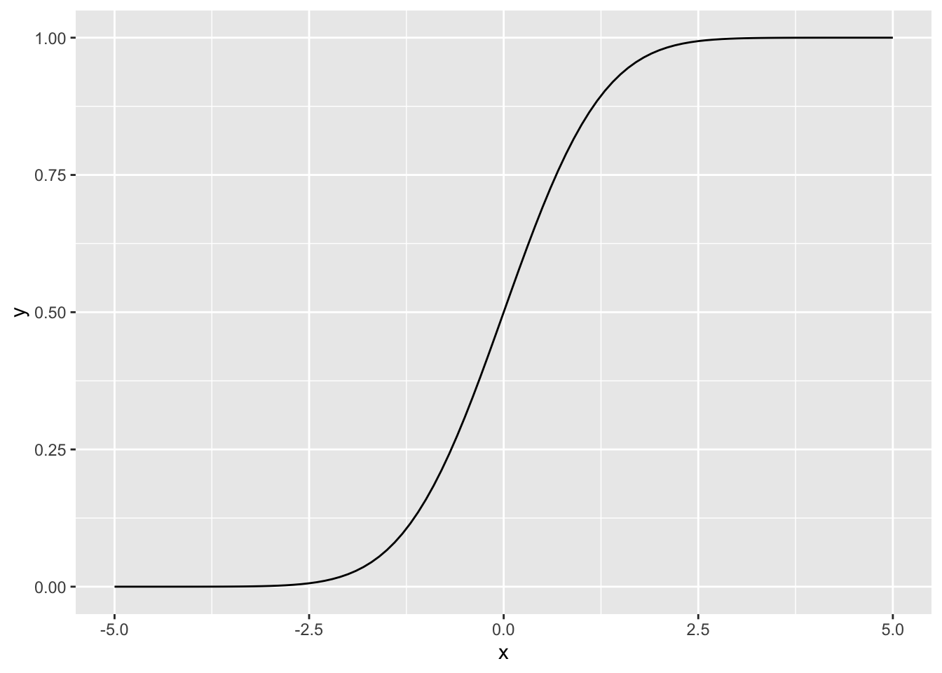

one_samp <- rnorm(1)
X        <- data.frame(x = c(-5, one_samp, 5), y = c(0,1,1))
ggplot(data = data.frame(x = seq(-5, 5, by = 0.01))) +
  # stat_function(aes(x = x), fun = pbeta, args = list(shape1 = 1, shape2 = 2))
  stat_function(aes(x = x), fun = pnorm, args = list(mean = 0, sd = 1)) +
  geom_step(data = X, aes(x = x, y = y))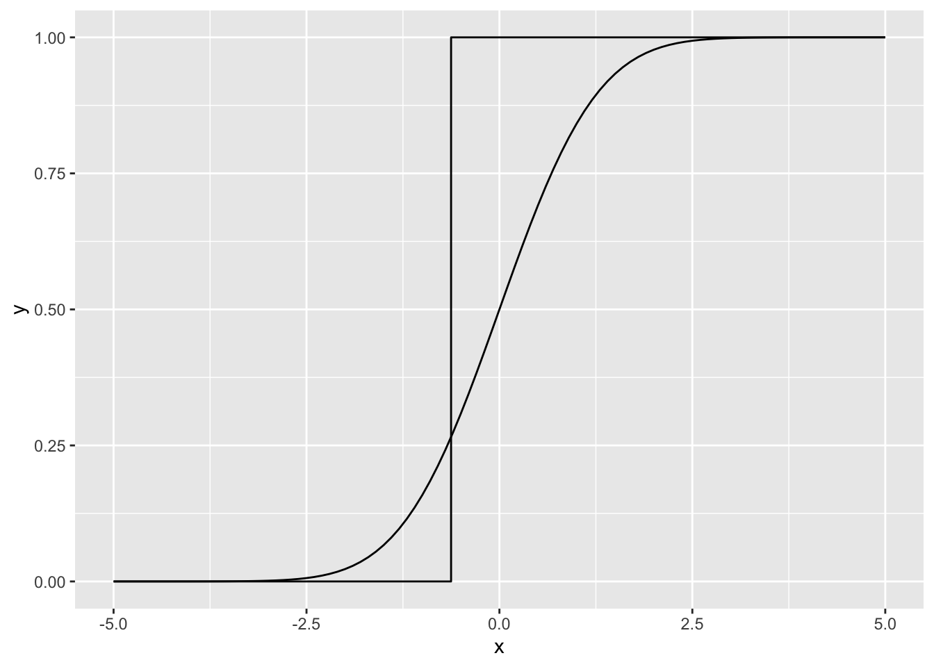

N <- c(5, 10, 100, 1000)
X <- NULL
for (n in N) {
  tmp   <- rnorm(n)
  tmp_X <- data.frame(x = c(-5, sort(tmp), 5), y = c(0, seq(1/n, 1, by = 1/n), 1), n = n)
  X     <- rbind(X, tmp_X)
}
ggplot(data = data.frame(x = seq(-5, 5, by = 0.01))) +
  # stat_function(aes(x = x), fun = pbeta, args = list(shape1 = 1, shape2 = 2))
  stat_function(aes(x = x), fun = pnorm, args = list(mean = 0, sd = 1)) +
  geom_step(data = X, aes(x = x, y = y, color = as.factor(n))) +
  labs(color = "N")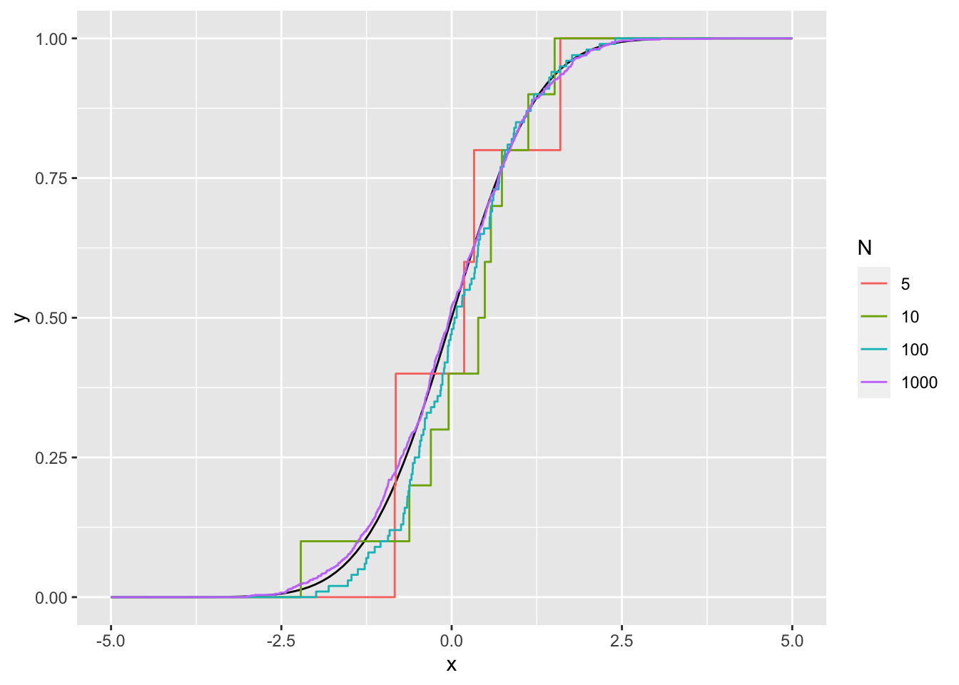

13.2 Properties of estimators

Exercise 13.2 Show that the sample average is, as an estimator of the mean:

unbiased,
consistent,
asymptotically normal.

Solution.

\[\begin{align*} E[\frac{1}{n} \sum_{i=1}^n X_i] &= \frac{1}{n} \sum_{i=i}^n E[X_i] \\ &= E[X]. \end{align*}\]
\[\begin{align*} \lim_{n \rightarrow \infty} P(|\frac{1}{n} \sum_{i=1}^n X_i - E[X]| > \epsilon) &= \lim_{n \rightarrow \infty} P((\frac{1}{n} \sum_{i=1}^n X_i - E[X])^2 > \epsilon^2) \\ & \leq \lim_{n \rightarrow \infty} \frac{E[(\frac{1}{n} \sum_{i=1}^n X_i - E[X])^2]}{\epsilon^2} & \text{Markov inequality} \\ & = \lim_{n \rightarrow \infty} \frac{E[(\frac{1}{n} \sum_{i=1}^n X_i)^2 - 2 \frac{1}{n} \sum_{i=1}^n X_i E[X] + E[X]^2]}{\epsilon^2} \\ & = \lim_{n \rightarrow \infty} \frac{E[(\frac{1}{n} \sum_{i=1}^n X_i)^2] - 2 E[X]^2 + E[X]^2}{\epsilon^2} \\ &= 0 \end{align*}\] For the last equality see the solution to ??.
Follows directly from the CLT.

Exercise 13.3 (Consistent but biased estimator)

Show that sample variance (the plug-in estimator of variance) is a biased estimator of variance.
Show that sample variance is a consistent estimator of variance.
Show that the estimator with (\(N-1\)) (Bessel correction) is unbiased.

Solution.

\[\begin{align*} E[\frac{1}{n} \sum_{i=1}^n (Y_i - \bar{Y})^2] &= \frac{1}{n} \sum_{i=1}^n E[(Y_i - \bar{Y})^2] \\ &= \frac{1}{n} \sum_{i=1}^n E[Y_i^2] - 2 E[Y_i \bar{Y}] + \bar{Y}^2)] \\ &= \frac{1}{n} \sum_{i=1}^n E[Y_i^2 - 2 Y_i \bar{Y} + \bar{Y}^2] \\ &= \frac{1}{n} \sum_{i=1}^n E[Y_i^2 - \frac{2}{n} Y_i^2 - \frac{2}{n} \sum_{i \neq j} Y_i Y_j + \frac{1}{n^2}\sum_j \sum_{k \neq j} Y_j Y_k + \frac{1}{n^2} \sum_j Y_j^2] \\ &= \frac{1}{n} \sum_{i=1}^n \frac{n - 2}{n} (\sigma^2 + \mu^2) - \frac{2}{n} (n - 1) \mu^2 + \frac{1}{n^2}n(n-1)\mu^2 + \frac{1}{n^2}n(\sigma^2 + \mu^2) \\ &= \frac{n-1}{n}\sigma^2 \\ < \sigma^2. \end{align*}\]
Let \(S_n\) denote the sample variance. Then we can write it as \[\begin{align*} S_n &= \frac{1}{n} \sum_{i=1}^n (X_i - \bar{X})^2 = \frac{1}{n} \sum_{i=1}^n (X_i - \mu)^2 + 2(X_i - \mu)(\mu - \bar{X}) + (\mu - \bar{X})^2. \end{align*}\] Now \(\bar{X}\) converges in probability (by WLLN) to \(\mu\) therefore the right terms converge in probability to zero. The left term converges in probability to \(\sigma^2\), also by WLLN. Therefore the sample variance is a consistent estimatior of the variance.
The denominator changes in the second-to-last line of a., therefore the last line is now equality.

Exercise 13.4 (Estimating the median)

Show that the sample median is an unbiased estimator of the median for N\((\mu, \sigma^2)\).
Show that the sample median is an unbiased estimator of the mean for any distribution with symmetric density.

Hint 1: The pdf of an order statistic is \(f_{X_{(k)}}(x) = \frac{n!}{(n - k)!(k - 1)!}f_X(x)\Big(F_X(x)^{k-1} (1 - F_X(x)^{n - k}) \Big)\).

Hint 2: A distribution is symmetric when \(X\) and \(2a - X\) have the same distribution for some \(a\).

Solution.

Let \(Z_i\), \(i = 1,...,n\) be i.i.d. variables with a symmetric distribution and let \(Z_{k:n}\) denote the \(k\)-th order statistic. We will distinguish two cases, when \(n\) is odd and when \(n\) is even. Let first \(n = 2m + 1\) be odd. Then the sample median is \(M = Z_{m+1:2m+1}\). Its PDF is \[\begin{align*} f_M(x) = (m+1)\binom{2m + 1}{m}f_Z(x)\Big(F_Z(x)^m (1 - F_Z(x)^m) \Big). \end{align*}\] For every symmetric distribution, it holds that \(F_X(x) = 1 - F(2a - x)\). Let \(a = \mu\), the population mean. Plugging this into the PDF, we get that \(f_M(x) = f_M(2\mu -x)\). It follows that \[\begin{align*} E[M] &= E[2\mu - M] \\ 2E[M] &= 2\mu \\ E[M] &= \mu. \end{align*}\] Now let \(n = 2m\) be even. Then the sample median is \(M = \frac{Z_{m:2m} + Z_{m+1:2m}}{2}\). It can be shown, that the joint PDF of these terms is also symmetric. Therefore, similar to the above \[\begin{align*} E[M] &= E[\frac{Z_{m:2m} + Z_{m+1:2m}}{2}] \\ &= E[\frac{2\mu - M + 2\mu - M}{2}] \\ &= E[2\mu - M]. \end{align*}\] The above also proves point a. as the median and the mean are the same in normal distribution.

Exercise 13.5 (Matrix trace estimation) The Hutchinson trace estimator [1] is an estimator of the trace of a symmetric positive semidefinite matrix A that relies on Monte Carlo sampling. The estimator is defined as \[\begin{align*} \textrm{tr}(A) \approx \frac{1}{n} \Sigma_{i=1}^n z_i^T A z_i, &\\ z_i \sim_{\mathrm{IID}} \textrm{Uniform}(\{-1, 1\}^m), & \end{align*}\] where \(A \in \mathbb{R}^{m \times m}\) is a symmetric positive semidefinite matrix. Elements of each vector \(z_i\) are either \(-1\) or \(1\) with equal probability. This is also called a Rademacher distribution.

Data scientists often want the trace of a Hessian to obtain valuable curvature information for a loss function. Per [2], an example is classifying ten digits based on \((28,28)\) grayscale images (i.e. MNIST data) using logistic regression. The number of parameters is \(m = 28^2 \cdot 10 = 7840\) and the size of the Hessian is \(m^2\), roughly \(6 \cdot 10^6\). The diagonal average is equal to the average eigenvalue, which may be useful for optimization; in MCMC contexts, this would be useful for preconditioners and step size optimization.

Computing Hessians (as a means of getting eigenvalue information) is often intractable, but Hessian-vector products can be computed faster by autodifferentiation (with e.g. Tensorflow, Pytorch, Jax). This is one motivation for the use of a stochastic trace estimator as outlined above.

References:

A stochastic estimator of the trace of the influence matrix for laplacian smoothing splines (Hutchinson, 1990)
A Modern Analysis of Hutchinson’s Trace Estimator (Skorski, 2020)

Prove that the Hutchinson trace estimator is an unbiased estimator of the trace.

Solution. We first simplify our task: \[\begin{align} \mathbb{E}\left[\frac{1}{n} \Sigma_{i=1}^n z_i^T A z_i \right] &= \frac{1}{n} \Sigma_{i=1}^n \mathbb{E}\left[z_i^T A z_i \right] \\ &= \mathbb{E}\left[z_i^T A z_i \right], \end{align}\] where the second equality is due to having \(n\) IID vectors \(z_i\). We now only need to show that \(\mathbb{E}\left[z^T A z \right] = \mathrm{tr}(A)\). We omit the index due to all vectors being IID: \[\begin{align} \mathrm{tr}(A) &= \mathrm{tr}(AI) \\ &= \mathrm{tr}(A\mathbb{E}[zz^T]) \\ &= \mathbb{E}[\mathrm{tr}(Azz^T)] \\ &= \mathbb{E}[\mathrm{tr}(z^TAz)] \\ &= \mathbb{E}[z^TAz]. \end{align}\] This concludes the proof. We clarify some equalities below.

The second equality assumes that \(\mathbb{E}[zz^T] = I\). By noting that the mean of the Rademacher distribution is 0, we have \[\begin{align} \mathrm{Cov}[z, z] &= \mathbb{E}[(z - \mathbb{E}[z])(z - \mathbb{E}[z])^T] \\ &= \mathbb{E}[zz^T]. \end{align}\] Dimensions of \(z\) are independent, so \(\mathrm{Cov}[z, z]_{ij} = 0\) for \(i \neq j\). The diagonal will contain variances, which are equal to \(1\) for all dimensions \(k = 1 \dots m\): \(\mathrm{Var}[z^{(k)}] = \mathbb{E}[z^{(k)}z^{(k)}] - \mathbb{E}[z^{(k)}]^2 = 1 - 0 = 1\). It follows that the covariance is an identity matrix. Note that this is a general result for vectors with IID dimensions sampled from a distribution with mean 0 and variance 1. We could therefore use something else instead of the Rademacher, e.g. \(z ~ N(0, I)\).

The third equality uses the fact that the expectation of a trace equals the trace of an expectation. If \(X\) is a random matrix, then \(\mathbb{E}[X]_{ij} = \mathbb{E}[X_{ij}]\). Therefore: \[\begin{align} \mathrm{tr}(\mathbb{E}[X]) &= \Sigma_{i=1}^m(\mathbb{E}[X]_{ii}) \\ &= \Sigma_{i=1}^m(\mathbb{E}[X_{ii}]) \\ &= \mathbb{E}[\Sigma_{i=1}^m(X_{ii})] \\ &= \mathbb{E}[\mathrm{tr}(X)], \end{align}\] where we used the linearity of the expectation in the third step.

The fourth equality uses the fact that \(\mathrm{tr}(AB) = \mathrm{tr}(BA)\) for any matrices \(A \in \mathbb{R}^{n \times m}, B \in \mathbb{R}^{m \times n}\).

The last inequality uses the fact that the trace of a \(1 \times 1\) matrix is just its element.