Chapter 9 Alternative representation of distributions
This chapter deals with alternative representation of distributions.
The students are expected to acquire the following knowledge:
Theoretical
- Probability generating functions.
- Moment generating functions.
9.1 Probability generating functions (PGFs)
Exercise 9.1 Show that the sum of independent Poisson random variables is itself a Poisson random variable. R: Let \(X\) be a sum of three Poisson distributions with \(\lambda_i \in \{2, 5.2, 10\}\). Take 1000 samples and plot the three distributions and the sum. Then take 1000 samples from the theoretical distribution of \(X\) and compare them to the sum.
Solution. Let \(X_i \sim \text{Poisson}(\lambda_i)\) for \(i = 1,...,n\), and let \(X = \sum_{i=1}^n X_i\). \[\begin{align} \alpha_X(t) &= \prod_{i=1}^n \alpha_{X_i}(t) \\ &= \prod_{i=1}^n \bigg( \sum_{j=0}^\infty t^j \frac{\lambda_i^j e^{-\lambda_i}}{j!} \bigg) \\ &= \prod_{i=1}^n \bigg( e^{-\lambda_i} \sum_{j=0}^\infty \frac{(t\lambda_i)^j }{j!} \bigg) \\ &= \prod_{i=1}^n \bigg( e^{-\lambda_i} e^{t \lambda_i} \bigg) & \text{power series} \\ &= \prod_{i=1}^n \bigg( e^{\lambda_i(t - 1)} \bigg) \\ &= e^{\sum_{i=1}^n \lambda_i(t - 1)} \\ &= e^{t \sum_{i=1}^n \lambda_i - \sum_{i=1}^n \lambda_i} \\ &= e^{-\sum_{i=1}^n \lambda_i} \sum_{j=0}^\infty \frac{(t \sum_{i=1}^n \lambda_i)^j}{j!}\\ &= \sum_{j=0}^\infty \frac{e^{-\sum_{i=1}^n \lambda_i} (t \sum_{i=1}^n \lambda_i)^j}{j!}\\ \end{align}\] The last term is the PGF of a Poisson random variable with parameter \(\sum_{i=1}^n \lambda_i\). Because the PGF is unique, \(X\) is a Poisson random variable.
set.seed(1)
library(tidyr)
nsamps           <- 1000
samps            <- matrix(data = NA, nrow = nsamps, ncol = 4)
samps[ ,1]       <- rpois(nsamps, 2)
samps[ ,2]       <- rpois(nsamps, 5.2)
samps[ ,3]       <- rpois(nsamps, 10)
samps[ ,4]       <- samps[ ,1] + samps[ ,2] + samps[ ,3]
colnames(samps)  <- c(2, 2.5, 10, "sum")
gsamps           <- as_tibble(samps)
gsamps           <- gather(gsamps, key = "dist", value = "value")
ggplot(gsamps, aes(x = value)) +
  geom_bar() +
  facet_wrap(~ dist)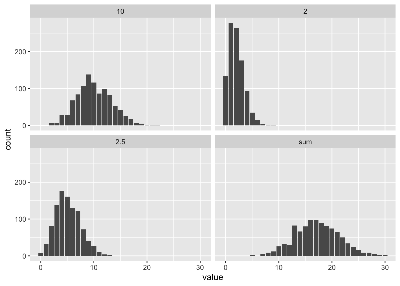
samps              <- cbind(samps, "theoretical" = rpois(nsamps, 2 + 5.2 + 10))
gsamps             <- as_tibble(samps[ ,4:5])
gsamps             <- gather(gsamps, key = "dist", value = "value")
ggplot(gsamps, aes(x = value, fill = dist)) +
  geom_bar(position = "dodge")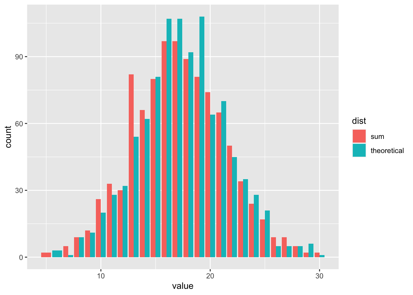
Exercise 9.2 Find the expected value and variance of the negative binomial distribution. Hint: Find the Taylor series of \((1 - y)^{-r}\) at point 0.
Solution. Let \(X \sim \text{NB}(r, p)\). \[\begin{align} \alpha_X(t) &= E[t^X] \\ &= \sum_{j=0}^\infty t^j \binom{j + r - 1}{j} (1 - p)^r p^j \\ &= (1 - p)^r \sum_{j=0}^\infty \binom{j + r - 1}{j} (tp)^j \\ &= (1 - p)^r \sum_{j=0}^\infty \frac{(j + r - 1)(j + r - 2)...r}{j!} (tp)^j. \\ \end{align}\] Let us look at the Taylor series of \((1 - y)^{-r}\) at 0 \[\begin{align} (1 - y)^{-r} = &1 + \frac{-r(-1)}{1!}y + \frac{-r(-r - 1)(-1)^2}{2!}y^2 + \\ &\frac{-r(-r - 1)(-r - 2)(-1)^3}{3!}y^3 + ... \\ \end{align}\] How does the \(k\)-th term look like? We have \(k\) derivatives of our function so \[\begin{align} \frac{d^k}{d^k y} (1 - y)^{-r} &= \frac{-r(-r - 1)...(-r - k + 1)(-1)^k}{k!}y^k \\ &= \frac{r(r + 1)...(r + k - 1)}{k!}y^k. \end{align}\] We observe that this equals to the \(j\)-th term in the sum of NB PGF. Therefore \[\begin{align} \alpha_X(t) &= (1 - p)^r (1 - tp)^{-r} \\ &= \Big(\frac{1 - p}{1 - tp}\Big)^r \end{align}\] To find the expected value, we need to differentiate \[\begin{align} \frac{d}{dt} \Big(\frac{1 - p}{1 - tp}\Big)^r &= r \Big(\frac{1 - p}{1 - tp}\Big)^{r-1} \frac{d}{dt} \frac{1 - p}{1 - tp} \\ &= r \Big(\frac{1 - p}{1 - tp}\Big)^{r-1} \frac{p(1 - p)}{(1 - tp)^2}. \\ \end{align}\] Evaluating this at 1, we get: \[\begin{align} E[X] = \frac{rp}{1 - p}. \end{align}\]
For the variance we need the second derivative. \[\begin{align} \frac{d^2}{d^2t} \Big(\frac{1 - p}{1 - tp}\Big)^r &= \frac{p^2 r (r + 1) (\frac{1 - p}{1 - tp})^r}{(tp - 1)^2} \end{align}\]
Evaluating this at 1 and inserting the first derivatives, we get: \[\begin{align} Var[X] &= \frac{d^2}{dt^2} \alpha_X(1) + \frac{d}{dt}\alpha_X(1) - \Big(\frac{d}{dt}\alpha_X(t) \Big)^2 \\ &= \frac{p^2 r (r + 1)}{(1 - p)^2} + \frac{rp}{1 - p} - \frac{r^2p^2}{(1 - p)^2} \\ &= \frac{rp}{(1 - p)^2}. \end{align}\]
library(tidyr)
set.seed(1)
nsamps <- 100000
find_p <- function (mu, r) {
  return (10 / (r + 10))
}
r <- c(1,2,10,20)
p <- find_p(10, r)
sigma <- rep(sqrt(p*r / (1 - p)^2), each = nsamps)
samps <- cbind("r=1"  = rnbinom(nsamps, size = r[1], prob = 1 - p[1]),
               "r=2"  = rnbinom(nsamps, size = r[2], prob = 1 - p[2]),
               "r=4"  = rnbinom(nsamps, size = r[3], prob = 1 - p[3]),
               "r=20" = rnbinom(nsamps, size = r[4], prob = 1 - p[4]))
gsamps <- gather(as.data.frame(samps))
iw     <- (gsamps$value > sigma + 10) | (gsamps$value < sigma - 10)
ggplot(gsamps, aes(x = value, fill = iw)) +
  geom_bar() +
  # geom_density() +
  facet_wrap(~ key)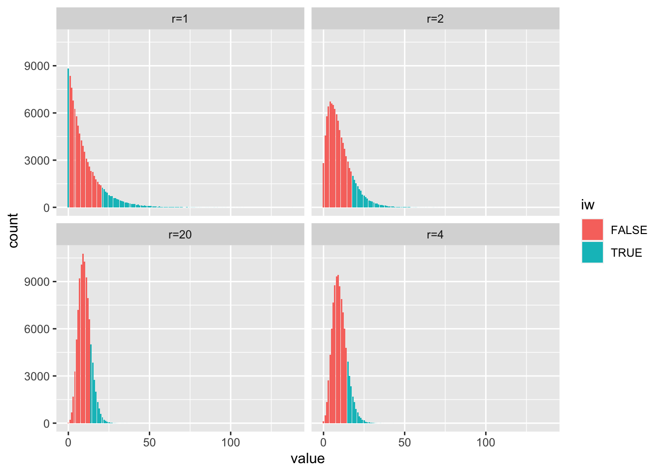
9.2 Moment generating functions (MGFs)
Exercise 9.3 Find the variance of the geometric distribution.
Solution. Let \(X \sim \text{Geometric}(p)\). The MGF of the geometric distribution is \[\begin{align} M_X(t) &= E[e^{tX}] \\ &= \sum_{k=0}^\infty p(1 - p)^k e^{tk} \\ &= p \sum_{k=0}^\infty ((1 - p)e^t)^k. \end{align}\] Let us assume that \((1 - p)e^t < 1\). Then, by using the geometric series we get \[\begin{align} M_X(t) &= \frac{p}{1 - e^t + pe^t}. \end{align}\] The first derivative of the above expression is \[\begin{align} \frac{d}{dt}M_X(t) &= \frac{-p(-e^t + pe^t)}{(1 - e^t + pe^t)^2}, \end{align}\] and evaluating at \(t = 0\), we get \(\frac{1 - p}{p}\), which we already recognize as the expected value of the geometric distribution. The second derivative is \[\begin{align} \frac{d^2}{dt^2}M_X(t) &= \frac{(p-1)pe^t((p-1)e^t - 1)}{((p - 1)e^t + 1)^3}, \end{align}\] and evaluating at \(t = 0\), we get \(\frac{(p - 1)(p - 2)}{p^2}\). Combining we get the variance \[\begin{align} Var(X) &= \frac{(p - 1)(p - 2)}{p^2} - \frac{(1 - p)^2}{p^2} \\ &= \frac{(p-1)(p-2) - (1-p)^2}{p^2} \\ &= \frac{1 - p}{p^2}. \end{align}\]
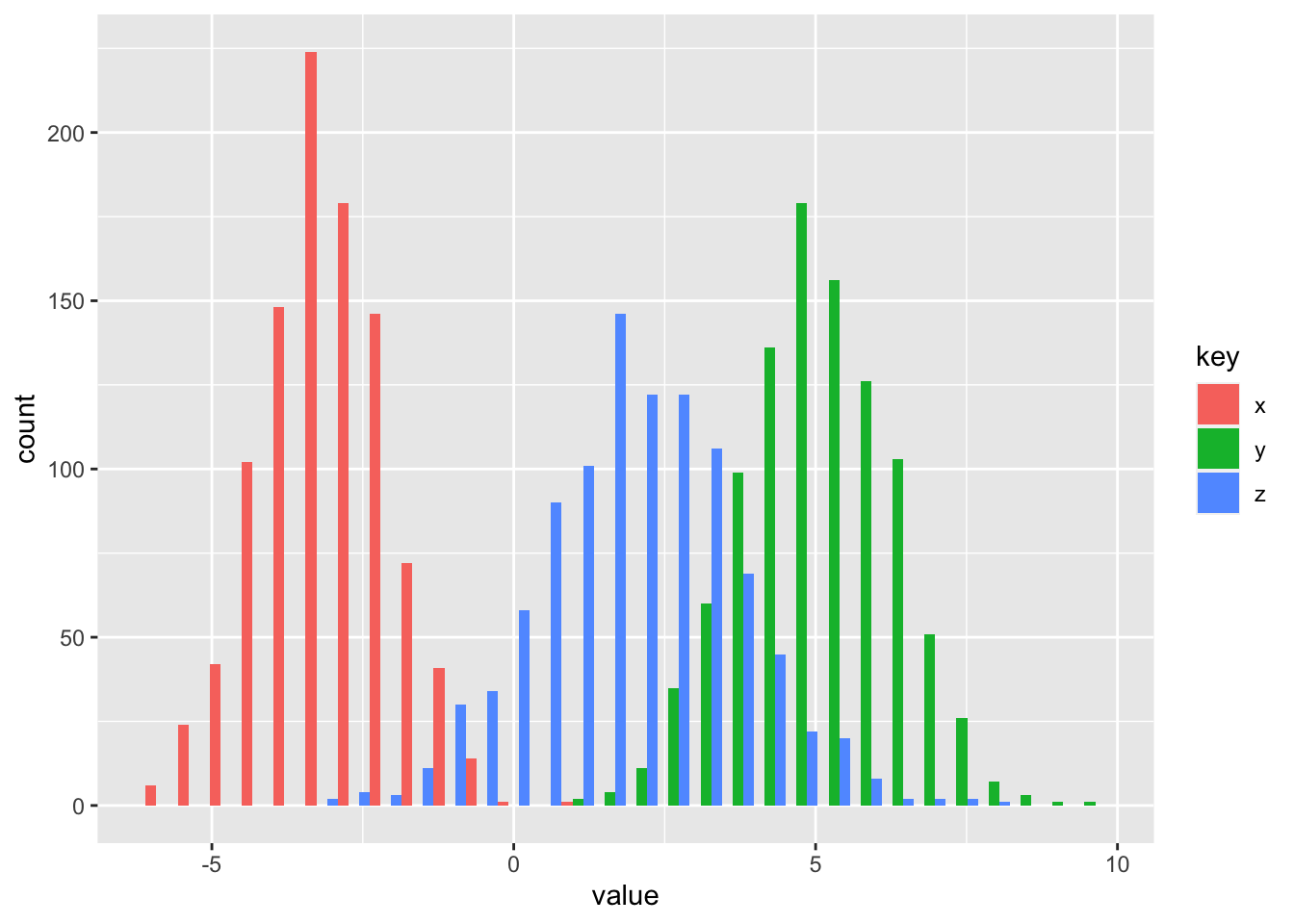
Exercise 9.4 Find the distribution of sum of two normal random variables \(X\) and \(Y\), by comparing \(M_{X+Y}(t)\) to \(M_X(t)\). R: To illustrate the result draw random samples from N\((-3, 1)\) and N\((5, 1.2)\) and calculate the empirical mean and variance of \(X+Y\). Plot all three histograms in one plot.
Solution. Let \(X \sim \text{N}(\mu_X, 1)\) and \(Y \sim \text{N}(\mu_Y, 1)\). The MGF of the sum is \[\begin{align} M_{X+Y}(t) &= M_X(t) M_Y(t). \end{align}\] Let us calculate \(M_X(t)\), the MGF for \(Y\) then follows analogously. \[\begin{align} M_X(t) &= \int_{-\infty}^\infty e^{tx} \frac{1}{\sqrt{2 \pi \sigma_X^2}} e^{-\frac{(x - mu_X)^2}{2\sigma_X^2}} dx \\ &= \int_{-\infty}^\infty \frac{1}{\sqrt{2 \pi \sigma_X^2}} e^{-\frac{(x - mu_X)^2 - 2\sigma_X tx}{2\sigma_X^2}} dx \\ &= \int_{-\infty}^\infty \frac{1}{\sqrt{2 \pi \sigma_X^2}} e^{-\frac{x^2 - 2\mu_X x + \mu_X^2 - 2\sigma_X tx}{2\sigma_X^2}} dx \\ &= \int_{-\infty}^\infty \frac{1}{\sqrt{2 \pi \sigma_X^2}} e^{-\frac{(x - (\mu_X + \sigma_X^2 t))^2 + \mu_X^2 - (\mu_X + \sigma_X^2 t)^2}{2\sigma_X^2}} dx & \text{complete the square}\\ &= e^{-\frac{\mu_X^2 - (\mu_X + \sigma_X^2 t)^2}{2\sigma_X^2}} \int_{-\infty}^\infty \frac{1}{\sqrt{2 \pi \sigma_X^2}} e^{-\frac{(x - (\mu_X + \sigma_X^2 t))^2}{2\sigma_X^2}} dx & \\ &= e^{-\frac{\mu_X^2 - (\mu_X + \sigma_X^2 t)^2}{2\sigma_X^2}} & \text{normal PDF} \\ &= e^{-\frac{\mu_X^2 - \mu_X^2 - \mu_X \sigma_X^2 t - 2 \sigma_X^4 t^2}{2\sigma_X^2}} \\ &= e^{\sigma_X^2 t^2 + \frac{\mu_X t}{2}}. \\ \end{align}\] The MGF of the sum is then \[\begin{align} M_{X+Y}(t) &= e^{\sigma_X^2 t^2 + 0.5\mu_X t} e^{\sigma_Y^2 t^2 + 0.5\mu_Y t} \\ &= e^{t^2(\sigma_X^2 + \sigma_Y^2) + 0.5 t(\mu_X + \mu_Y)}. \end{align}\] By comparing \(M_{X+Y}(t)\) and \(M_X(t)\) we observe that both have two terms. The first is \(2t^2\) multiplied by the variance, and the second is \(2t\) multiplied by the mean. Since MGFs are unique, we conclude that \(Z = X + Y \sim \text{N}(\mu_X + \mu_Y, \sigma_X^2 + \sigma_Y^2)\).
library(tidyr)
library(ggplot2)
set.seed(1)
nsamps <- 1000
x      <- rnorm(nsamps, -3, 1)
y      <- rnorm(nsamps, 5, 1.2)
z      <- x + y
mean(z)
## [1] 1.968838## [1] 2.645034df <- data.frame(x = x, y = y, z = z) %>%
gather()
ggplot(df, aes(x = value, fill = key)) +
geom_histogram(position = "dodge")