Chapter 9 Relational databases
Organizations, researchers and other individuals have been using databases to store and work with data since they exist. Software that implements a specific database is called a database management system. It provides a complete software solution to work with data and implements security, consistency, simultaniety, administration, etc. There exist different types of database management systems, depending on the type of data they store - for example relational, object, document, XML, noSQL, etc. In this section we focus on the relational databases which provide a common interface using the SQL query language – a common basic query language, which we use for searching and manipulating data in relational databases. Example database management systems are Oracle, IBM DB2, MSSQL, MySQL, PostgreSQL or SQLite.
Relational model implemented by the relational databases represents the database as a collection of relations. Relation as defined in theory is most easily represented as a table (note that a concept of a relation is not a table!). Tuple of data is represented as a row. Generally each row describes an entity, e.g. a person. Each tuple contains a number of columns/attributes. Each value is defined within a domain of possible values. Special fields (e.g. primary key) define relational integrity constraints, that is conditions which must be present for a valid relation. Constraints on the Relational database management system is mostly divided into three main categories are (a) domain constraints, (b) key constraints and (c) referential integrity constraints. An example of a relation representation is shown in the Figure below.
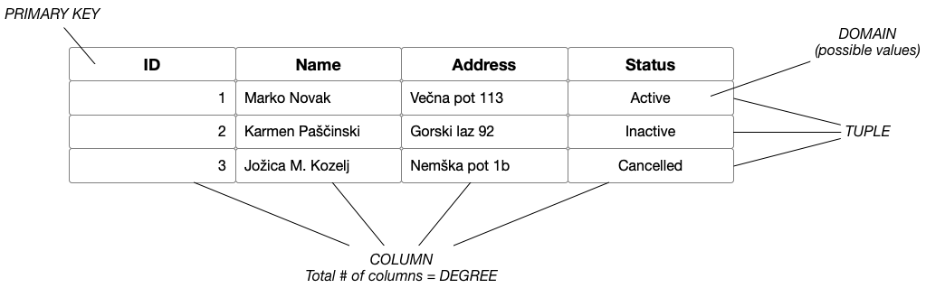
Figure 6.1: Relation representation.
9.1 Introduction to SQL
Structure Query Language (SQL), pronounced as “sequel” is a domain-specific language used in programming and designed for managing data held in a relational database management system. It is based on relational algebra and tuple relational calculus. SQL consists of many types of statements, such as a data manipulation language, a data definition language or a data control language. Although SQL is a declarative language, its extensions include also procedural elements. SQL became a standard in 1986 and has been revised a few times since to include new features. Despite the existence of standards, most SQL code is not completely portable among different database systems.
For the data scientist, data modelling and querying are the most important. We will focus only on these two aspects of the SQL which are also the most common to all database systems. In order to use advanced mechanisms such as security management, procedural functionalities or locking, please review the documentation of your selected database system.
9.1.1 Data definition language
Data definition language SQL sentences enable us to manipulate with the structure of the database. They define SQL data types and provide mechanisms to manipulate with database objects, data quality assertion mechanisms, transactions and definition of procedural objects such as procedures and functions.
The data types of data columns in tables are defined as follows (ANSI SQL):
| Type | SQL data types |
|---|---|
| binary | BIT, BIT VARYING |
| time | DATE, TIME, TIMESTAMP |
| number | DECIMAL, REAL, DOUBLE PRECISION, FLOAT, SMALLINT, INTEGER, INTERVAL |
| text | CHARACTER, CHARACTER VARYING, NATIONAL CHARACTER, NATIONAL CHARACTER VARYING |
Many database management systems can host multiple schemas or databases, so we need first to create the database using CREATE DATABASE DatabaseName. After that we need to explicity say which database will be used by the following commands using USE DatabaseName. If we do not issue that command, we need to addres every database object as DatabaseName.ObjectName.
To create new tables, we use the CREATE TABLE statement, which looks as follows:
CREATE TABLE TableName (
    {colName dataType [NOT NULL] [UNIQUE]
    [DEFAULT defaultOption]
    [CHECK searchCondition] [,...]}
    [PRIMARY KEY (listOfColumns),]
    {[UNIQUE (listOfColumns),] [...,]}
    {[FOREIGN KEY (listOfFKColumns)
       REFERENCES ParentTableName [(listOfCKColumns)],
       [ON UPDATE referentialAction]
       [ON DELETE referentialAction ]] [,...]}
    {[CHECK (searchCondition)]})
Constraints are useful, because they allow the database’s referential integrity protection to take care of data correctness. With the command NULL or NOT NULL we define that a column may or may not contain a missing value. The parameter UNIQUE defines a constraint on a specific column that must not contain duplicated values in the whole table. We can also define it separately for more columns at once, similarly to the primary key syntax.
Using this statement we can also define column specifics, such as data type, constraints, foreign keys or primary keys. All of these can be changed later using ALTER commands. For example, to drop an existing constraint or foreign key, we use:
To add a new integer-type column that must not be undefined and has a specific default value if not set to database, we issue:
When we create a table, an index is created for the columns that represent the primary key. There exist a number of different indexes, which are various and implemented differently across the database management systems. Indexes can improve our query performances but are costly to build and can consume a lot of space, so they need to be created wisely when needed. To create an index, we use the following syntax:
CREATE [UNIQUE|FULLTEXT|SPATIAL] INDEX index_name
   ON table_name
      (column1 [ASC|DESC],
       column2 [ASC|DESC],
...);
To delete a database object, a DROP command is used. Using a DROP command we can delete any database object or a whole database. To delete a table, we use following command:
Analogously, the command is used for constraints, indexes, users, databases, etc. In the example above we see two additional arguments - RESTRICT and CASCADE. They specifically define, whether the table can be deleted if there exist some columns in other tables that reference columns in the table we wish to delete.
9.1.2 Data manipulation language
When a database and tables or other objects are created, we can focus on inserting, updating, deleting and querying data.
9.1.2.1 Inserting
Statements for inserting rows into a database table looks as follows:
The list of columns is not necessary if we provide all the columns in the same order that were defined at the table creation time. In the data values we need to provide at least all the values that are of NOT NULL type and do not have the default value set. The order of values in the list need correspond to the column list.
To insert more rows at a time, multiple data value lists can be used. When doing a bulk inserts, this will speed up our insertion time. To insert enormous amounts of data into relational database, some database management systems provide their own mechanisms of bulk data importing, as well as for data export.
9.1.2.2 Updating
The UPDATE statements allows us to change values within the existing data rows. It is defined as follows:
UPDATE TableName
SET columnName1 = dataValue1
   [, columnName2 = dataValue2...]
[WHERE searchCondition]
We can update one or more column values in the selected table. The statement will update all the rows that initially satisfy the search condition. The search condition is optional but we must take care when updating or deleting rows as our command may change too many rows if search condition not defined correctly.
9.1.2.3 Deleting
Statement for deleting rows is similar to updating without setting new values. The sentence deletes all the rows in a table that match the search condition is defined as follows:
9.1.2.4 Querying
Querying is enabled by the SELECT statement which is the most comprehensive as provides multiple mechanisms to access the data from a database:
SELECT [DISTINCT | ALL] {* | [columnExpression [AS newName]] [,...] }
FROM
  TableName [alias] [, ...]
[JOIN table2 [alias2] ON condition]
[WHERE condition]
[GROUP BY columnList]
[HAVING condition]
[ORDER BY columnList [ASC|DESC]]
In the SELECT part we can define whether the returned results must be distinct or not. Then we list columns that should be returned as the result. The columns may be named or changed using a special function provided by a database management system (DBMS). Some DBMS also support nested SELECT statements in this part when statement returns only one value.
In the FROM part we list tables that are needed for the query to execute. It is possible to nest a SELECT statement instead of using a table - write a query within brackets and give it an alias. Depending on our needs we can use joins in this part to connect the rows between tables. To see which joins are supported by a specific DBMS, we need to check its documentation.
In the WHERE part we provide conditions that need to be true for the row to be returned. In this part we can use equality operators (>, <, =, <=, >=, BETWEEN), text comparisons (LIKE), set comparisons (IN, ALL, ANY), null value comparisons (IS NULL, IS NOT NULL) or specific functions supported by our DBMS.
The GROUP BY part groups together rows of the same value by the defined columns. On this group of columns we can run further aggregate functions. When using grouping, we can output only columns that are grouped by or aggregate functions of other columns in the SELECT part! Use with caution as some DBMS do not provide warnings if grouping used wrongly. Standard aggregate functions are COUNT, SUM, AVG, MIN and MAX. Each DBMS provides also additional grouping functions such as GROUP_CONCAT (MySQL specific, other databases name proprietary functions differently).
The HAVING part can be used only together with GROUP BY. Its role is to provide filtering of rows based on the aggregate functions - these cannot be used in the WHERE part of the query.
In the last part we define the order of returned results. By default, the order of rows is undefined.
9.1.2.5 Query Order of Execution
The order of execution in SQL defines the sequence in which a query’s components are evaluated. While SQL queries are written in a human-readable, declarative style, the underlying database engine processes them in a systematic order to retrieve results efficiently. Understanding this order is crucial for writing correct and optimized queries.
The order is as follows:
- FROM: Identify and retrieve data from the tables or views specified.
- JOIN: Combine data from multiple tables based on the join conditions.
- WHERE: Filter rows based on specified conditions before any grouping or aggregation.
- GROUP BY: Group the filtered data into buckets based on column values.
- HAVING: Filter groups created by
GROUP BYbased on aggregate functions. - SELECT: Retrieve specified columns or calculated results from the remaining data.
- ORDER BY: Sort the final result set.
- LIMIT: Restrict the number of rows returned in the result set.
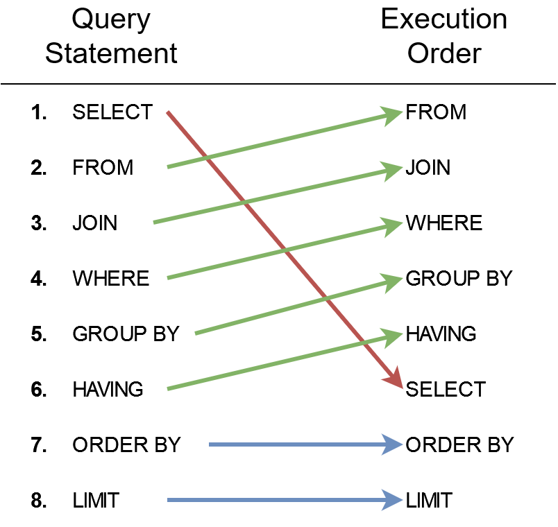
Figure 9.1: Order of SQL query execution.
9.2 SQLite
In the previous part we pointed out some basics about data management in relational databases. In this part we will show SQL in practice using an SQLite database.
SQLite is an open source, zero-configuration, self-contained, stand-alone, transaction relational database engine designed to be embedded into an application. This type of the database is used by our desktop applications, mobile applications, etc. and it does not need a special server-based database management system. Its structure is contained in a special file, which can be handled by a sqlite database management library.
Sqlite seems like a simple database implementation. It lacks performance over large amounts of data, reliability, scalability, redundancy, concurrent access/transactions and other advanced features such as referential integrity, special indexing capabilities and functions, procedural SQL, etc. In the case of data science needs we often need a database only as a simple data storage that is better than storing the data in raw files. Therefore the choice of SQLite of our main database would be enough for the most of our needs.
9.2.1 Environment setup
To install an SQLite database we just do need to download a binary version from the official SQLite web site. There exist also installation packages that install SQLite program to our computer and update the $PATH variable so that the sqlite command is directly accessible from command line.
The sqlite 3 download package consists of three executables:
sqldiff: The utility that displays the differences between SQLite databases.sqlite3: The main executable to create and manage SQLite databases.sqlite3_analyzer: The utility that outputs a human-readable ASCII text report which provides information on the space utilization of the database file.
To start working with a database, just run the sqlite3 command in the command-line:
$ sqlite3
SQLite version 3.23.1 2018-04-10 17:39:29
Enter ".help" for usage hints.
Connected to a transient in-memory database.
Use ".open FILENAME" to reopen on a persistent database.
sqlite>
We exit the console by entering the CTRL+C command twice. The example above created just a temporary database in our memory, so no data was stored on disk. To work with or create a new database if not exists, we need to provide a filename when starting the executable - sqlite3 itds_course.db. When we change the defaults of the database or enter some data, the database file will be created.
There exist a lot of standalone graphical user interfaces to work with SQLite database files. An example of a nice and lightweight software to create, open or manage SQLite databases is DB Browser for SQLite and is available for multiple operating systems.
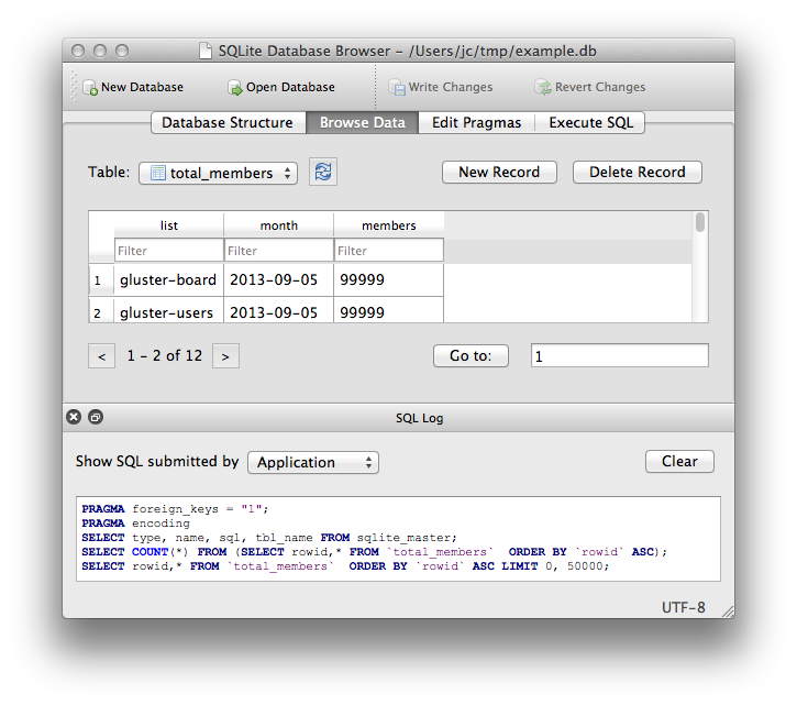
Figure 9.2: DB Browser for SQLite graphical user interface.
9.2.2 SQLite database usage
In this section we show how to create a new SQLite database and manage it manually using SQL language directly. First we create a new database file called itds_course.db.
We will create a new database model, presented in the Figure 9.3. Modeling database schemas can be a complex task, especially for larger databases consisting of many tables. The modeler needs to follow rules, needs to know how the database will be used, the approximate frequency of data insertion, most common queries, etc. Generally, we first prepare a conceptual model, which is easily understandable to laypersons. Then we create a logical model which contains specifics of a database - foreign keys, constraints, indexes, etc. Lastly, a pyhsical model or SQL script is created to instantiate a database on a selected database management system. Model changes in a live database later can be quite more difficult than at the beginning.
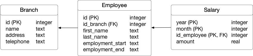
Figure 9.3: Employee logical database model.
Let’s first create the model from the Figure 9.3. The model consists of three tables - Branch, Employee and Salary. Employees must be employed at one of the branches and can get a salary each month. In the model some basic restrictions are defined, such as primary and foreign keys and data types. The data types are related to the SQLite database, which does not support many different types. Therefore time-based attributes are represented as text.
SQLite supports foreign keys but it does not enforce their referential integrity if we do not say this explicitly at each database connection session. To enable checks, we need to issue the following command:
-- Set the foreign keys checking on
PRAGMA foreign_keys = ON;
-- Check the foreign keys setting (1=ON, 0=OFF)
PRAGMA foreign_keys;
We observe that, by default, each SQL statement is terminated using a semicolon. Now we can continue and create all the tables:
-- Creating Branch table
CREATE TABLE Branch (
    id INTEGER PRIMARY KEY AUTOINCREMENT,
    name TEXT NOT NULL,
    address TEXT NOT NULL,
    telephone TEXT
);

-- Employee
CREATE TABLE Employee (
    id INTEGER PRIMARY KEY AUTOINCREMENT,
    id_branch INTEGER NOT NULL,
    first_name TEXT NOT NULL,
    last_name TEXT NOT NULL,
    employment_start TEXT NOT NULL,
    employment_end TEXT,
    FOREIGN KEY (id_branch) REFERENCES Branch(id)
);

-- Salary
CREATE TABLE Salary (
    year INTEGER,
    month INTEGER,
    id_employee INTEGER,
    amount REAL NOT NULL,
    PRIMARY KEY (year, month, id_employee),
    FOREIGN KEY (id_employee) REFERENCES Employee(id)
);
When creating tables, we should be consistent in naming them - capitalization, singular/plural and similarly for the columns, especially foreign keys. The most readable tables have clearly identifiable primary key and foreign keys. Naming of the foreign key columns should reflect the name of the related table. In the Branch and Employee tables we defined the primary key columns as AUTOINCREMENT. This enables the database to automatically set the id of a new record and we do not need to define it explicitly.
Now we can insert some data into our tables. The insertion into the Employee table could be done also using one statement only. For the still employed employees we would just set their employment_end value to NULL.
-- Branches
INSERT INTO Branch (name, address, telephone) VALUES
    ("Grosuplje's Fried Chicken", "Kolodvorska 1, Grosuplje", "01/786-42-31");
INSERT INTO Branch (name, address) VALUES
    ("Hot Pork Wings", "Cesta v Kranj 35, Ljubljana");

-- Employees (still employed)
INSERT INTO Employee (id_branch, first_name, last_name, employment_start) VALUES
    (1, "Marko", "Novaković", "1972-01-25"),
    (1, "Jože", "Novak", "1995-08-22"),
    (1, "Janez", "Gruden", "1999-12-07"),
    (1, "Tine", "Stegel", "2002-04-28"),
    (1, "Nina", "Gec", "2010-03-08"),
    (1, "Petar", "Stankovski", "2018-10-01");

-- Employees (retired)
INSERT INTO Employee (id_branch, first_name, last_name, employment_start, employment_end) VALUES
    (1, "Jana", "Žitnik", "1987-06-07", "1987-06-12"),
    (1, "Patricio", "Rozman", "2010-04-22", "2022-01-01"),
    (1, "Robert", "Demšar", "1996-12-06", "1997-07-02");

-- Salaries
INSERT INTO Salary (year, month, id_employee, amount) VALUES
    (2010, 05, 2, 950.37),
    (2010, 06, 2, 955.2),
    (2010, 07, 2, 990.49),
    (2010, 08, 2, 1200.5),
    (2010, 05, 6, 980.43),
    (2010, 05, 7, 1320.2),
    (2010, 05, 8, 2100.67),
    (2010, 06, 8, 2140.99),
    (2010, 07, 8, 2099.11);
Now the data are in the database and we can query them. Below we show just some basic queries. The command-line output does not include column names, so when they are not defined in the query, their order is as in the table.
1|Grosuplje's Fried Chicken|Kolodvorska 1, Grosuplje|01/786-42-31
2|Hot Pork Wings|Cesta v Kranj 35, Ljubljana|
-- Selecting a column with a condition
SELECT employment_start
FROM Employee
WHERE last_name = "Gec";-- Result value concatenation
SELECT id, first_name || ' ' || last_name AS name
FROM Employee
WHERE employment_end IS NULL;SQLite also supports advanced querying, for example:
- Show the number of employees and a maximum salary for each branch.
-- Grouping and aggregations
SELECT b.id, b.name, COUNT(e.id), MAX(s.amount)
FROM Branch b, Employee e, Salary s
WHERE
    e.id_branch = b.id AND
    s.id_employee = e.id
GROUP BY b.id, b.name;- The query above does not return branches with no employees, which is not expected. To improve the query, we need to introduce outer joins. They enable outputs even if there are no matching records in a related table. You may think also of other solutions to solve the problem.
-- Grouping and outer joins
SELECT b.id, b.name, COUNT(e.id), MAX(s.amount)
FROM Branch b LEFT OUTER JOIN Employee e ON e.id_branch = b.id
     LEFT OUTER JOIN Salary s ON s.id_employee = e.id
GROUP BY b.id, b.name;- Select all the employees that got their salary even though they were not employed any more by a branch. Instead of using data from a table directly, we pre-prepare the data using a nested query which is used then in the same way as a new table in a query.
-- Nested select statement
SELECT *
FROM (SELECT e.id, e.first_name, e.last_name, s.amount, e.employment_end, s.year, s.month
      FROM Employee e, Salary s
      WHERE
         e.id = s.id_employee AND
         e.employment_end IS NOT NULL) t
WHERE
    strftime('%Y', t.employment_end) < t.year OR
    (strftime('%Y', t.employment_end) = t.year AND
strftime('%m', t.employment_end) < t.month);Sometimes we would like our results of a query to be stored into a new table. We can achieve this using a CREATE AS statement. The example above prepares a table with all the employees and their salaries that we can further analyse using data science methods:
CREATE TABLE SalaryAnalysis AS
SELECT e.id, e.employment_start, e.employment_end,
       s.year || '-' || s.month || '-01' AS month, s.amount
FROM Employee e INNER JOIN Salary s ON e.id = s.id_employee;

SELECT * FROM SalaryAnalysis;2|1995-08-22||2010-5-01|950.37
2|1995-08-22||2010-6-01|955.2
2|1995-08-22||2010-7-01|990.49
2|1995-08-22||2010-8-01|1200.5
6|2018-10-01||2010-5-01|980.43
7|1987-06-07|1987-06-12|2010-5-01|1320.2
8|2010-04-22|2022-01-01|2010-5-01|2100.67
8|2010-04-22|2022-01-01|2010-6-01|2140.99
8|2010-04-22|2022-01-01|2010-7-01|2099.11Another option is to create a dynamic object called VIEW. The CREATE VIEW command assigns a name to a pre-packaged SELECT statement. Once the view is created, it can be used in the FROM clause of another SELECT in place of a table name. We can also rename columns when creating a view. We now use the same example as above to create a VIEW:
CREATE VIEW SalaryAnalysisView (id, start, end, month, amount) AS
SELECT e.id, e.employment_start, e.employment_end,
       s.year || '-' || s.month || '-01' AS month, s.amount
FROM Employee e INNER JOIN Salary s ON e.id = s.id_employee;

SELECT * FROM SalaryAnalysisView;2|1995-08-22||2010-5-01|950.37
2|1995-08-22||2010-6-01|955.2
2|1995-08-22||2010-7-01|990.49
2|1995-08-22||2010-8-01|1200.5
6|2018-10-01||2010-5-01|980.43
7|1987-06-07|1987-06-12|2010-5-01|1320.2
8|2010-04-22|2022-01-01|2010-5-01|2100.67
8|2010-04-22|2022-01-01|2010-6-01|2140.99
8|2010-04-22|2022-01-01|2010-7-01|2099.11There is also option to update our data using the UPDATE statement:
-- Set new phone number to the Hot Pork Wings branch
UPDATE Branch
 SET telephone = "05/869-22-54"
 WHERE name = "Hot Pork Wings";

-- Retire the Employee 3 starting today
UPDATE Employee
 SET employment_end = date('now')
 WHERE id = 3;
DELETE statements are similar to UPDATE statements. In both cases we must be careful about the WHERE condition as we may quickly delete or update too many rows.
The statement above could not delete Employees as there exist rows in the Salary table that refer to the rows in the Employee table. Therefore, we need to first delete the rows from the Salary table and then from the Employee table. More advanced databases support the CASCADE mechanism in the DELETE statement already which can be used for such scenarios.
DELETE FROM Salary WHERE id_employee IN (
    SELECT id FROM Employee WHERE employment_end IS NOT NULL
);

DELETE FROM Employee WHERE employment_end IS NOT NULL;
We presented just some basic examples of how to use an SQLite database. Feel free to investigate its possibilities further.
9.2.3 SQLite in Python
SQLite can be used by many different programming languages. We show an example of how to use an SQLite database from Python. The database we prepared in the previous section is also available here.
First we need to install library for SQLite database file manipulation. If you use Anaconda Python distribution, just issue the conda install -c anaconda sqlite command.
Then we need to connect to a database. If the database file does not exist in the path provided, an empty database file will be created automatically.
9.2.3.1 Inserting data
We assume that we are connected to the database from the previous section. Let’s first insert a record.
c = conn.cursor()

c.execute('''
    INSERT INTO Employee (id_branch, first_name, last_name, employment_start) VALUES
      (2, "Mija", "Zblaznela", "1999-07-12");
''')

c.execute('''
    INSERT INTO Salary (year, month, id_employee, amount) VALUES
      (2010, 05, last_insert_rowid(), 1243.67);
''')


# Save (commit) the changes
conn.commit()

# We can also close the connection if we are done with it.
# Just be sure any changes have been committed or they will be lost.
# conn.close()
After every change to a database, we must call the commit command which actually saves the results into the database.
Now let’s examine if our insert statement was successful. You may have noticed the call to the function last_insert_rowid(). This function returns the id of the last inserted row when we are using AUTOINCREMENT option for the primary key.
9.2.3.2 Selecting data
Let’s check, what is in the database.
cursor = c.execute('''
    SELECT b.id, b.name, COUNT(e.id), MAX(s.amount)
    FROM Branch b LEFT OUTER JOIN Employee e ON e.id_branch = b.id
         LEFT OUTER JOIN Salary s ON s.id_employee = e.id
    GROUP BY b.id, b.name;
''')

for row in cursor:
    print("\tBranch id: %d\n\t\tBranch name: '%s'\n\t\tEmployee number: \
    %s\n\t\tMaximum salary: %s" % (row[0], row[1], row[2], row[3]))

# You should close the connection when stopped using the database.
conn.close()
We can observe that now also the Hot Pork Wings branch employs an employee.
9.3 PostgreSQL
In some cases we need more powerful relational database features. In this case we propose to use a more advanced relational database management system, such as PostgreSQL, MS SQL, MySQL or others.
In previous chapters we introduced Docker environment. Now we will use an official PostgreSQL database image and run it:
The command will run a PostgreSQL v10.0 database in a Docker container. Also, it will name the container pg-server, set the default database user’s postgres’ password to BeReSeMi.DataScience and share the port 5432 to the host machine.
When the container is running, we can use our preffered database client and connect to the database server. We can also directly connect to the database using the following command:
First we need to create a database, called courseitds and connect to it:
postgres=# create database courseitds;
CREATE DATABASE
postgres=# \c courseitds
You are now connected to database "courseitds" as user "postgres".
Now we can use the SQL statements from the example above (Section 9.2.2). PostgreSQL supports SQL a bit differently, so we need to adapt the following:
- Foreign key constraint checks are enabled by default so there is no need to enable them.
- The command AUTOINCREMENT is not supported. We can use a data type SERIAL which already includes the functionality. Foreign keys can still be of INTEGER type.
- Dates can used the data type DATE. Also functions for querying are different. For example,
EXTRACT (YEAR FROM t.employment_end)extracts a year value from a date. - We should not use double quotes for values. Therefore we change all double quotes to single quotes. Single quotes that are part of a value should be escaped with an additional single quote.
We provided adapted SQL queries in a single SQL file.
When running a database using Docker, do not forget about the data storage! Using the container storage directly is not safe, so we should use volumes instead.
9.4 Further reading and references
- SQLite official website and Sqlite 3 Python library documentation.
- There are lots of SQLite tutorial, such as SQLite tutorial.net.
- PostgreSQL official documentation.
9.5 Learning outcomes
Data science students should work towards obtaining the knowledge and the skills that enable them to:
- Use SQL to model, query and update a relational database.
- Setup a relational database and use it from your programming language of choice.
- Import and export data to and from a database.
9.6 Practice problems
- Select one of the machine learning datasets, design a database for it and import it into a database. Use the Python visualization library and visualize the data queried directly from the database.
- Adapt the examples from above for use with another relational database management system - e.g. MySQL, MSSQL or Oracle.
- Go through SQL hands-on tutorial and practise using SQL (SQLite and PostgreSQL). Think of different options, such as using other database, domain, …